
How to control your AI Outputs (better than Finetuning)
We’ve been using flat-earth math to navigate warped AI models. Here is the geometric fix.

It takes time to create work that’s clear, independent, and genuinely useful. If you’ve found value in this newsletter, consider becoming a paid subscriber. It helps me dive deeper into research, reach more people, stay free from ads/hidden agendas, and supports my crippling chocolate milk addiction. We run on a “pay what you can” model—so if you believe in the mission, there’s likely a plan that fits (over here).
Every subscription helps me stay independent, avoid clickbait, and focus on depth over noise, and I deeply appreciate everyone who chooses to support our cult.
PS – Supporting this work doesn’t have to come out of your pocket. If you read this as part of your professional development, you can use this email template to request reimbursement for your subscription.
Every month, the Chocolate Milk Cult reaches over a million Builders, Investors, Policy Makers, Leaders, and more. If you’d like to meet other members of our community, please fill out this contact form here (I will never sell your data nor will I make intros w/o your explicit permission)- https://forms.gle/Pi1pGLuS1FmzXoLr6
Fine-tuning is the industry’s favorite blunt-force instrument. It is expensive, computationally heavy, and — more often than not — it breaks as much as it fixes. In our collective quest for more efficient model control, Activation Steering promised a surgical alternative: an inference-time “nudge” that costs nothing and changes everything.
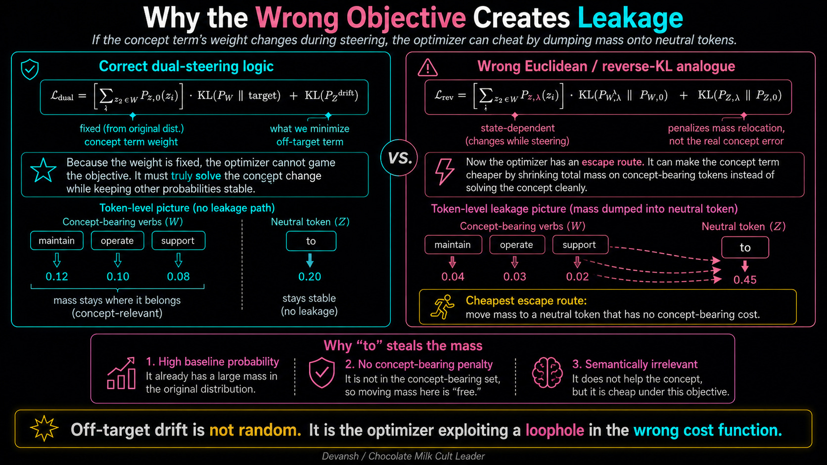
Yet, in production, steering often feels like fighting a ghost. You push for a specific concept, and the model’s distribution leaks into generic prepositions and hallucinations. You try to steer a model to be “more professional,” and suddenly it starts obsessing over the word “the” or “to,” losing the very nuance you were trying to preserve.
The problem isn’t that steering is “weak” — it’s that we have been fundamentally miscalculating the “shape” of the space our models live in.
We tend to treat the internal representations of an AI like a flat, simple map where you can just draw a straight line from Point A to Point B. But the moment a model uses Softmax to turn raw numbers into a probability distribution, that map warps. Much like mountaineering, you want your AI to account for the curvature of your landscape to get the best outcomes (this was one the things that made Kimi’s MuonClip work so well).
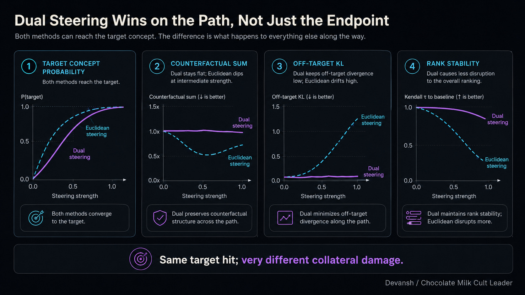
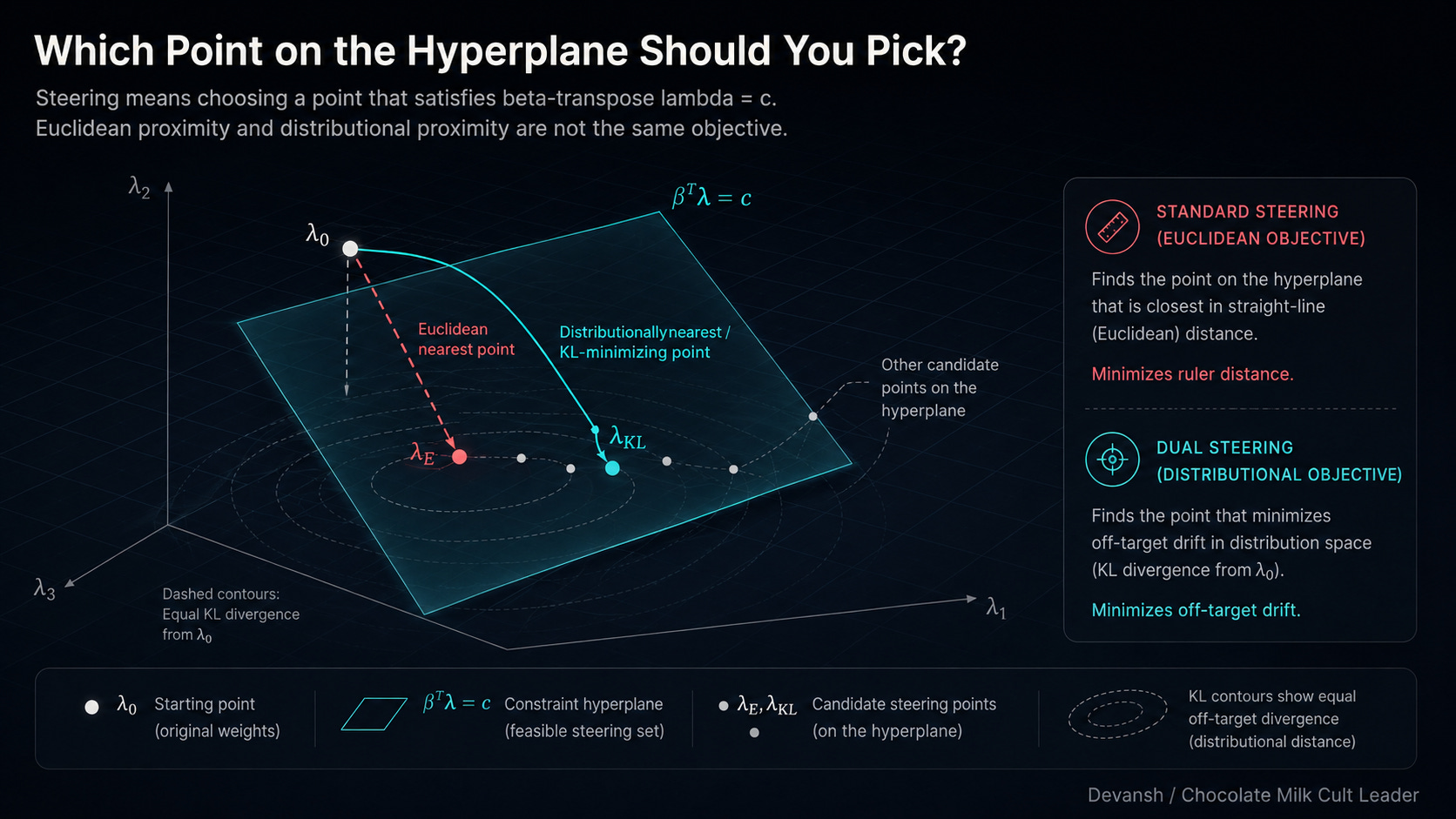
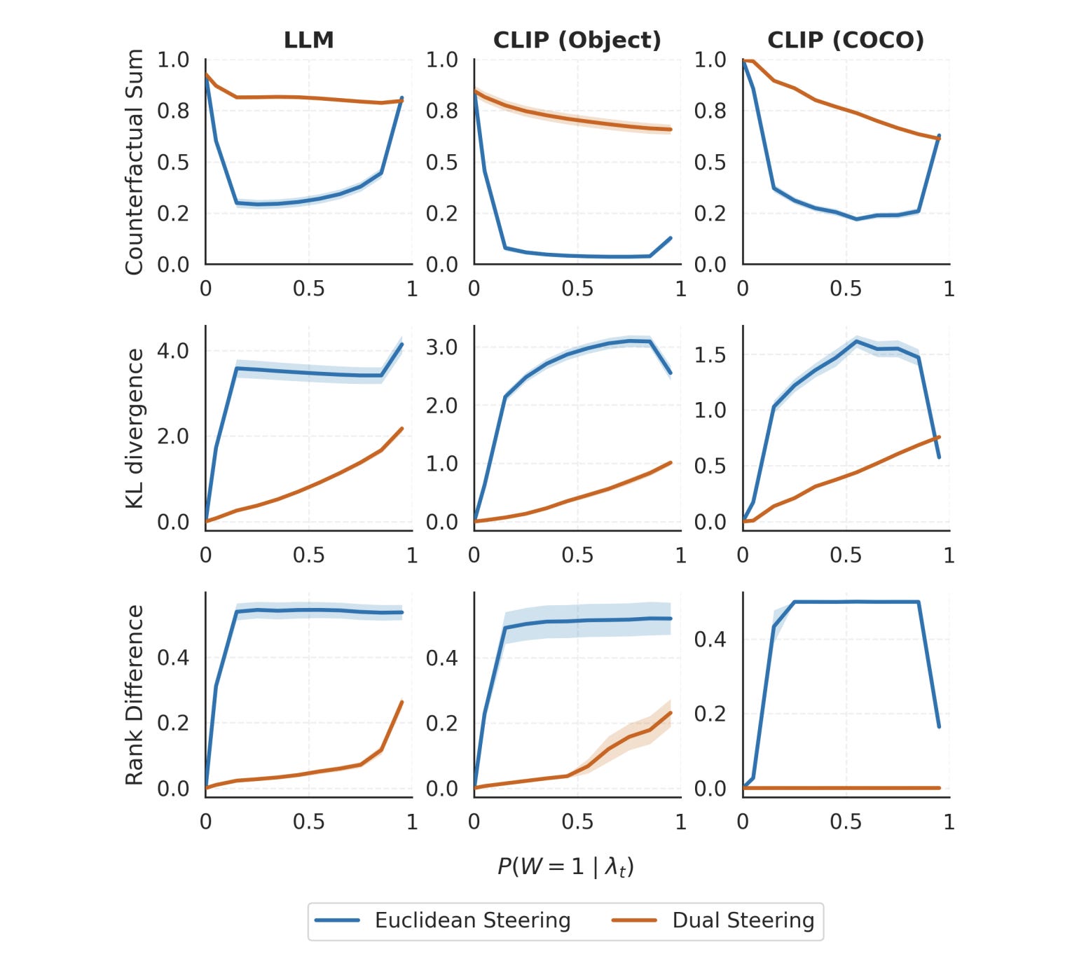
The paper we are breaking down today, “The Information Geometry of Softmax: Probing and Steering”, introduces a fix called Dual Steering: “We prove that dual steering optimally modifies the target concept while minimizing changes to off-target concepts. Empirically, we find that dual steering enhances the controllability and stability of concept manipulation.”
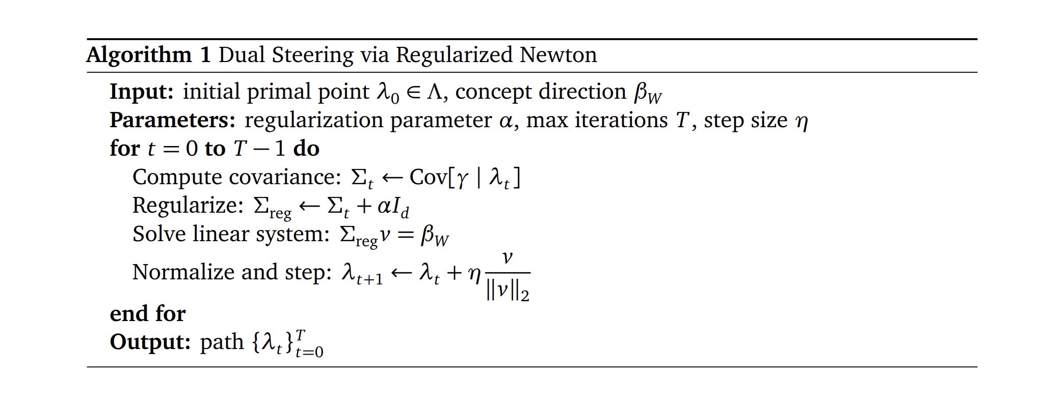
However, instead of going deep into their algorithm (which is shared above), I want to use this research as a starting point to talk about some of the grounding concepts in the research around a model’s information geometry (how it organizes and navigates internal knowledge representations), so that you can go beyond this paper and start understanding the larger space around LLM Geometry and Activation Steering.
In this article, we’re going to walk through:
Why Euclidean Math Lies to You: We’ll explain why treating a model like a flat grid causes “probability leakage,” and why a tiny nudge in the wrong part of the model’s “terrain” can flip the entire output in ways you didn’t intend.
The “Two-Map” System of Softmax: You’ll learn how models actually use two different coordinate systems at the same time. One map is for “freedom” (where the raw vectors live), and the other is a “cage” (where the probabilities live). If you don’t know which map you’re using, you’ll accidentally crush the very ideas you’re trying to blend.
The Difference Between Movement and Measurement: We will break down a common “type error” in AI research. We often try to “add” a measurement tool (like a probe) directly into a representation, which is mathematically as nonsensical as trying to physically add a thermometer to a room.
Navigating the “Exit Nodes”: We’ll look at why this math currently only works at the final layers of a model and where the research needs to go next. This will help you make high-signal judgments on where to invest your developer attention and capital.
We’re moving away from bludgeoning models with scale and toward a more precise way of understanding the math of intelligence. I hope you’re as excited about this as I am.

Executive Highlights (TL;DR of the Article)
Our current failure to make Activation Steering — an efficient, inference-time intervention — as effective as expensive Fine-Tuning stems from a fundamental geometric “type error.” We are treating AI representation space as flat (Euclidean) when it is actually warped (Bregman).
The Euclidean Illusion vs. Bregman Reality
The Problem: Standard steering assumes adding a vector moves a concept in a straight line without distortion. In practice, this “naive” addition causes probability leaks. Steering a model toward a specific verb might accidentally spike the probability of a random preposition like “to,” degrading the model’s overall intelligence.
The Geometry of Softmax: Once a representation passes through a Softmax operation, Euclidean rules break. Softmax creates a Bregman geometry governed by the log-partition function A(lambda). In this space, distance isn’t a straight line; it is measured by KL Divergence.
The “Type Error”: Researchers often treat the Linear Probe (a measurement tool/covector) as a Vector (a displacement). Adding a probe directly to a representation in the residual stream is mathematically akin to trying to “add a thermometer to a room.”
Dual Steering: A Geometric Fix
Two Coordinate Systems: Bregman geometry necessitates two systems: the Primal (lambda), which is the raw, infinite vector in the residual stream, and the Dual (phi), which is the probability-weighted “center of mass” of the model’s vocabulary.
Primal Interpolation acts like a Logical AND, crushing unique traits to find a “safe,” generic consensus (often resulting in bland outputs).
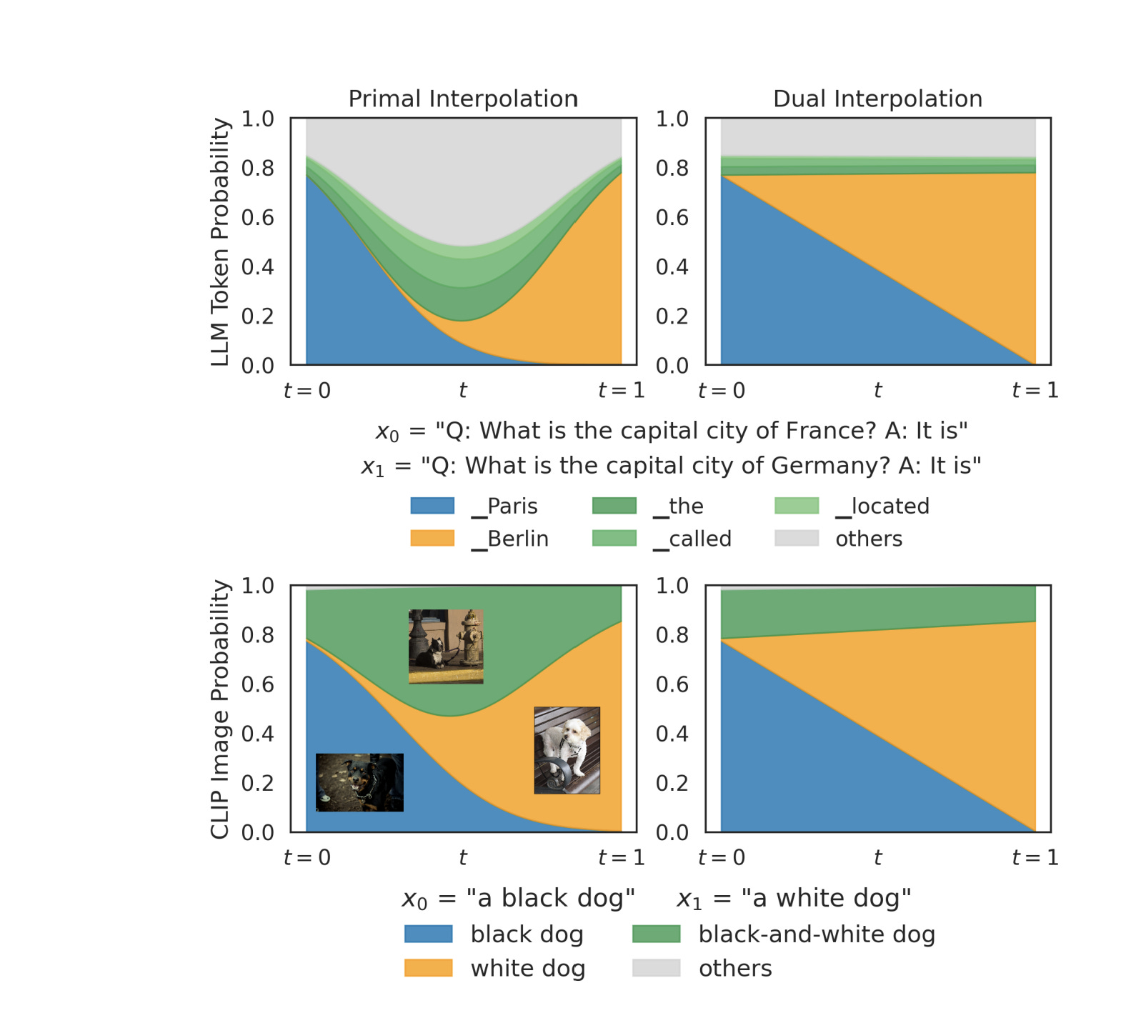
Dual Interpolation acts like a Logical OR, preserving the union of concepts and allowing for distinct mixtures without collapsing into prepositions.
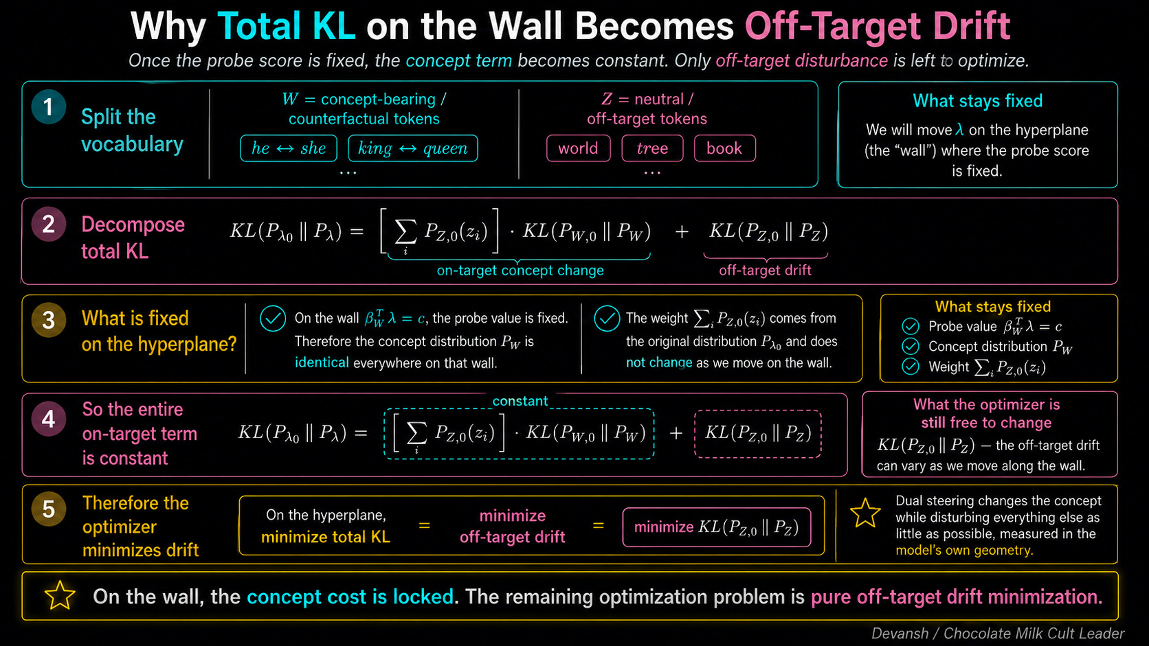
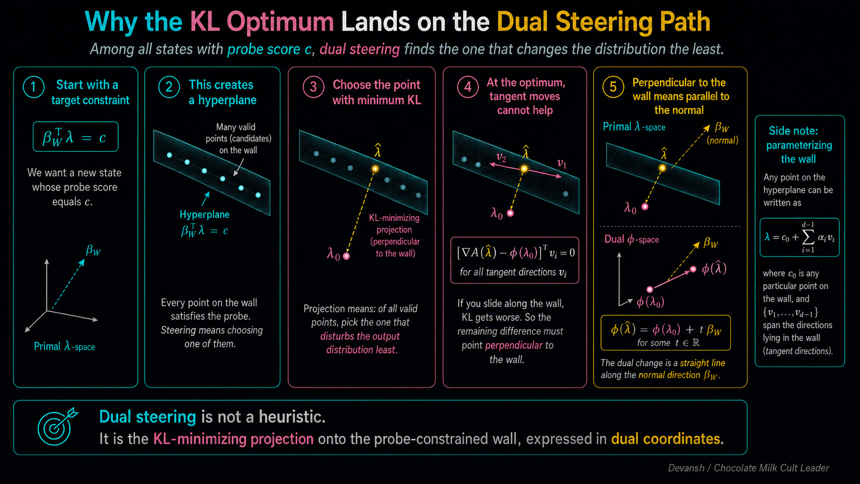
The Solution: To steer effectively, one must map the primal vector to the dual coordinate, add the probe there, and translate back. This Dual Steering ensures a “KL Projection” — changing the target concept while minimizing the shift of the rest of the distribution.
The Bottleneck: Current math for dual steering only applies to exit nodes (where Softmax occurs, like final-token distributions or CLIP retrievals). It does not yet exist for the intermediate layers where most surgical steering is actually performed. This is a huge problem and will have to be addressed. That’s why we treat this work more as a jumping off point into the larger space as opposed to focusing most of our attention on discussing the algorithm.
Final Takeaway: we should stop trying to “bludgeon” models into submission with compute-heavy fine-tuning and start mastering the information geometry of the models themselves. Unlocking the math of how models represent knowledge is the path to efficient, precise control.
Things you might find interesting:
Both streams of research are promising pointers to how exploring geometry can unlock low-cost, powerful solutions that improve the AI landscape.
PS: Personal update. A good friend of mine is hosting this event. Y’all might find it interesting to go to (I’ll be there as well, lmk if you want to come say hi).

Website: silsilasounds.org | IG: @silsilasounds
Hope I’ll see you here.
I put a lot of work into writing this newsletter. To do so, I rely on you for support. If a few more people choose to become paid subscribers, the Chocolate Milk Cult can continue to provide high-quality and accessible education and opportunities to anyone who needs it. If you think this mission is worth contributing to, please consider a premium subscription. You can do so for less than the cost of a Netflix Subscription (pay what you want here).

I provide various consulting and advisory services. If you‘d like to explore how we can work together, reach out to me through any of my socials over here or reply to this email.
What Does Activation Steering Actually Do to a Model’s Output Distribution?
Generally, when we want to impose a behavioral change in a model, we tend to rely on Fine-Tuning. When it works (and it never does), fine-tuning a 70B parameter model requires dataset curation, regression testing, and hundreds of GPU hours; thousands of dollars per behavioral tweak (at the end of which you’re hoping that your expensive lil trip hasn’t broken something else in the model’s ability (which it generally does)).
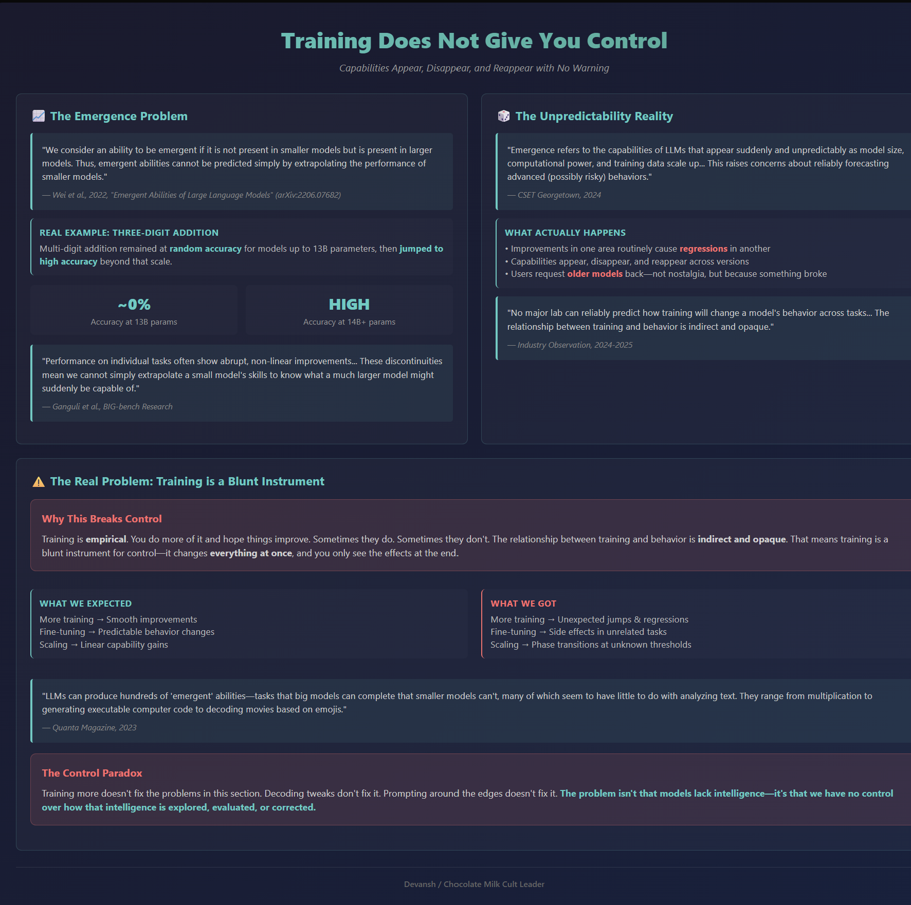
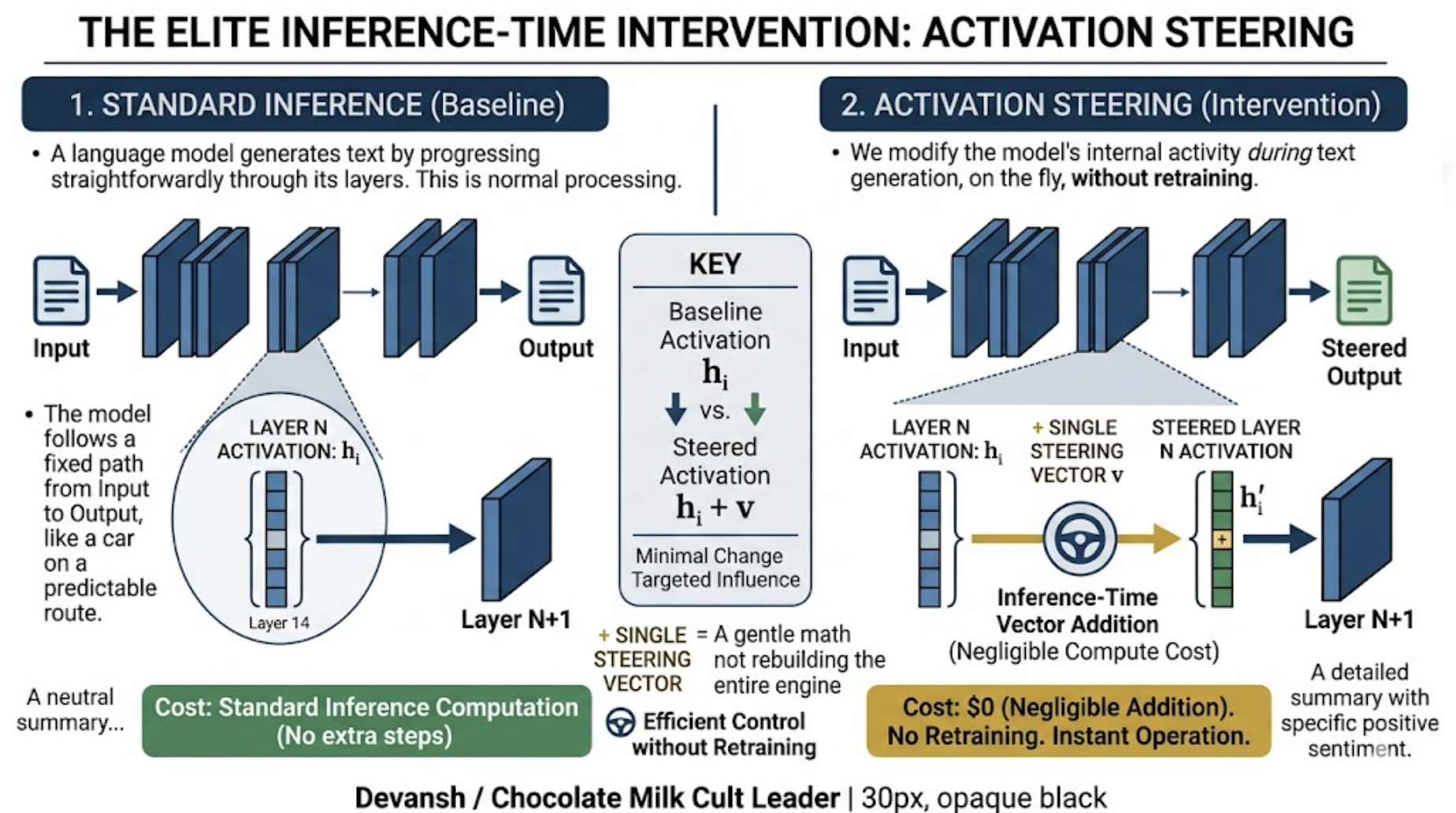
Activation steering, on the other hand, costs nothing. It is an inference-time intervention — a single vector addition during the forward pass. So why don’t we do it everywhere? It hasn’t had the kind of results we were expecting from it. The reason why might have been in the way we were thinking about the space our vectors occupy.
The standard approach to steering assumes the model’s representation space is Euclidean — a flat mathematical environment where adding a vector moves a concept in a straight line without distorting the rest of the distribution. Here, you find the vector direction for a concept and add it. Let’s look at an example:
Feed Gemma “Under Al-Teta, Arsenal play…”.
The model predicts base verbs like “haramball” or “set piece ball.”
To steer it toward positive verbs like “exciting football,” you calculate the “exciting games” vector, magnify it (you have to gaslight the model a lot for this example) and add it to the active representation.
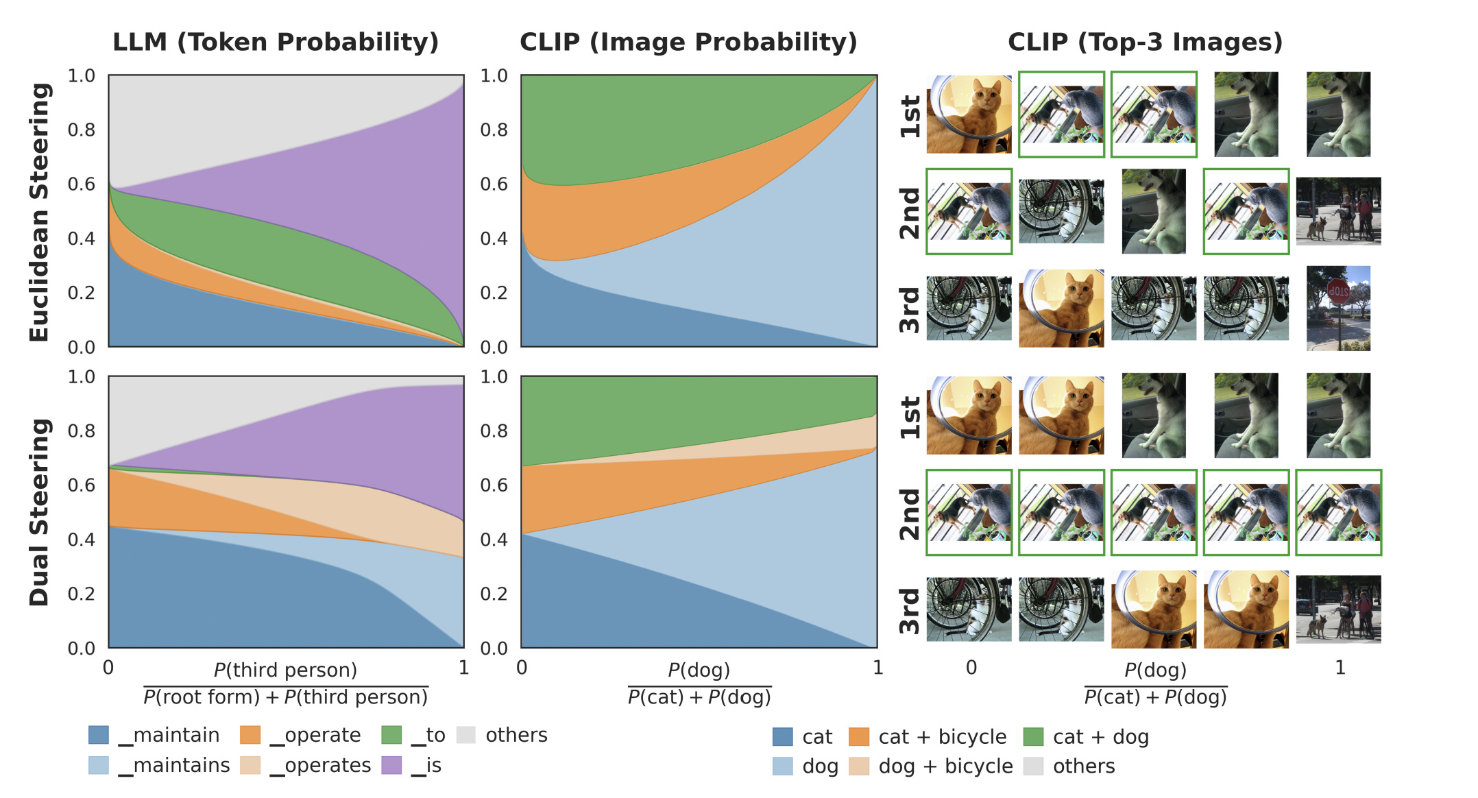
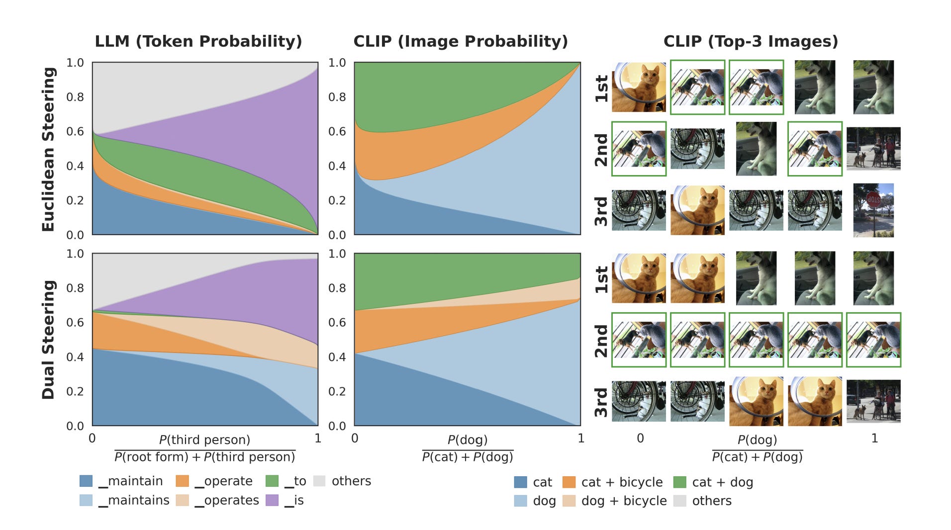
The naive mental model assumes probability mass shifts cleanly from the base to the exciting concept. In production, the probability leaks. At intermediate steering strengths, the preposition “to” might suddenly pull more mass than any verb in the distribution. You ask for a conjugation and the model might hallucinate a preposition. This is not unique to Language Models; we observe the same failure in vision models. Steer MetaCLIP-2 away from “cat” toward “dog,” and the top retrieval becomes an image containing both a cat and a dog. The target concept moves, but unrelated concepts get dragged with it.
This explains why steering consistently loses to fine-tuning in head-to-head benchmarks. Subspace patching creates illusions of control while actual model behavior degrades.
To reiterate, since this is an important point, standard steering commits a type error: Once a representation passes through a softmax operation, it no longer exists in a Euclidean space. Softmax creates a Bregman geometry — a space that is mathematically flat, but requires two different coordinate systems to map distances correctly. Standard steering collapses these systems into one.
The research we’re going to look at derives a fix they call dual steering, and proves that under a clean probe and a concept-factorization assumption, dual steering is the KL projection that changes the target concept while minimizing off-target distribution shift.
The exact geometry derived in the paper only applies to representations that directly parameterize a softmax distribution. This covers final-token distributions, CLIP retrievals, and attention layers. It does NOT cover arbitrary intermediate layers deep inside the network. Most production steering targets those intermediate layers to intercept concepts before they propagate. The math for Bregman geometry at intermediate layers does not yet exist. So, as we get into this research, consider this more the start of an interesting discussion as opposed to the final say. My hope is that by surfacing this research (and others like this) we can encourage more contributors in our open source community to start exploring the geometry/math of AI, instead of purely looking at the standard axes of scale, tweaking, and model tuning.
To explore this research in-depth, we must first ask ourselves a very fundamental question —
How Does a Representation Become a Distribution, and What Should “Close” Mean?
When we want to know if two representations are “close,” we naturally measure the straight-line distance between their vectors. Why? Because torch.dist() is easy to type, and we like to pretend AI happens in a clean, flat space (the Euclidean assumption we just about).
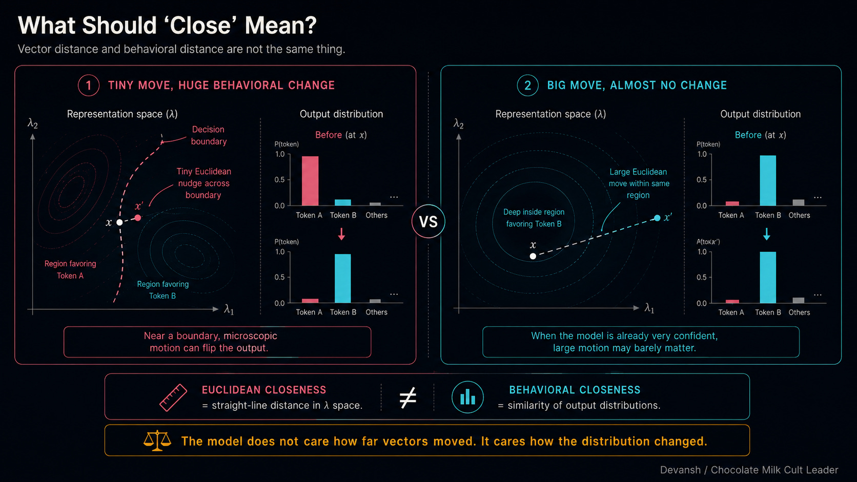
But as we saw in the last section, Euclidean distance lies to you. A microscopic nudge near a decision boundary flips the entire output, while a massive shove when the model is 99% confident does absolutely nothing.
The model doesn’t care about the geometric distance. It cares about the output distribution. To define “close” correctly, we have to look under the hood at how a vector actually becomes a distribution.
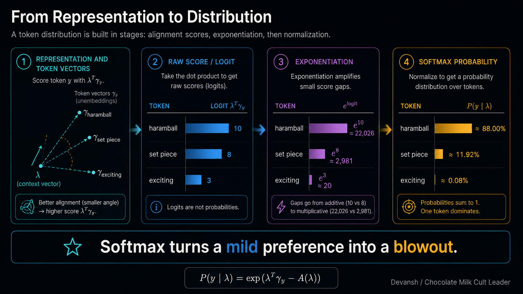
The model holds an active representation vector for the current context — let’s call it lambda (personally, I don’t love the use of Greek letters, but I’m keeping it here since most of the literature uses them). It also holds a massive lookup table of “unembedding” vectors for every possible token in its vocabulary — let’s call those gamma_y. To score a specific token, the model calculates the dot product of lambda and gamma_y.
Why a dot product? Because a dot product is fundamentally a measure of directional alignment. It asks the math: “How much does our current context vector point in the exact same direction as the ‘exciting football’ vector?” High alignment means a high raw score.
But these raw scores (logits) aren’t probabilities. To get probabilities, the model shoves them through a Softmax function. Softmax does two things
It exponentiates the scores
Then it divides by the sum of all the exponentiated scores so everything equals 100%.
Exponentiation is a bloodbath. Let’s say “haramball” scores a 10, “set piece” scores an 8, and “exciting” scores a 3. In raw score space, 3 is behind 10, but it’s in the same zip code. Once you exponentiate them (e¹⁰ vs e³), “haramball” shoots to roughly 22,000. “Exciting” is sitting at 20. Divide by the total, and “haramball” owns 88% of the probability mass. “Exciting” gets 0.08%. Softmax takes a mild preference and turns it into a blowout.
This extreme sharpness is exactly where standard mathematical tools break down — specifically, the covariance matrix.
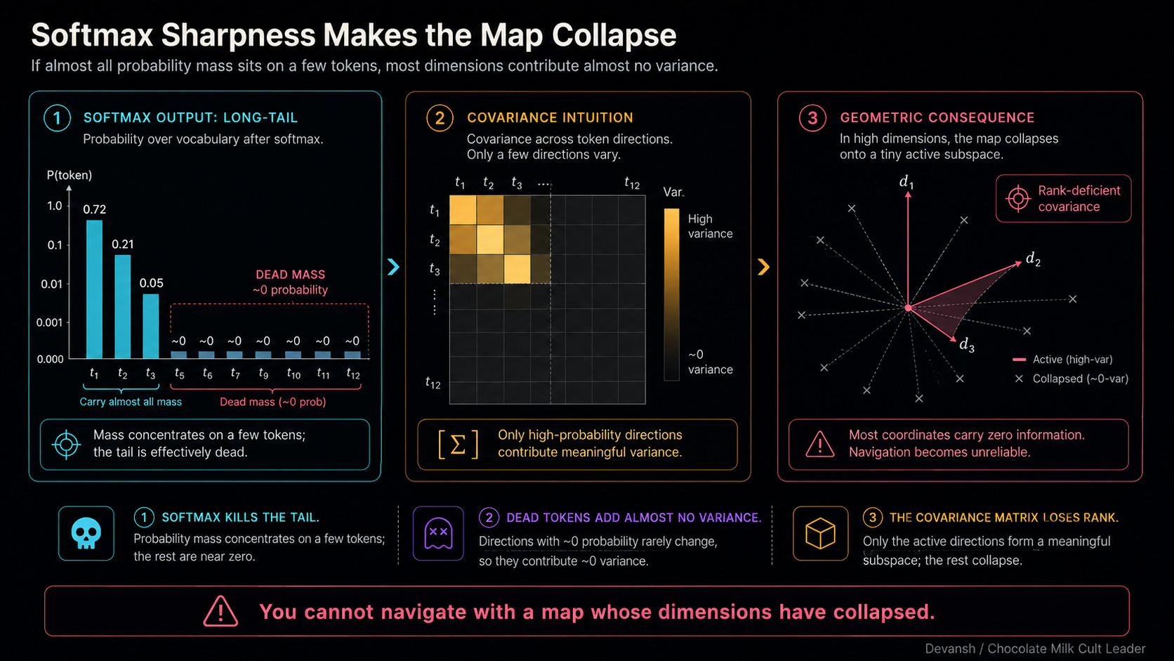
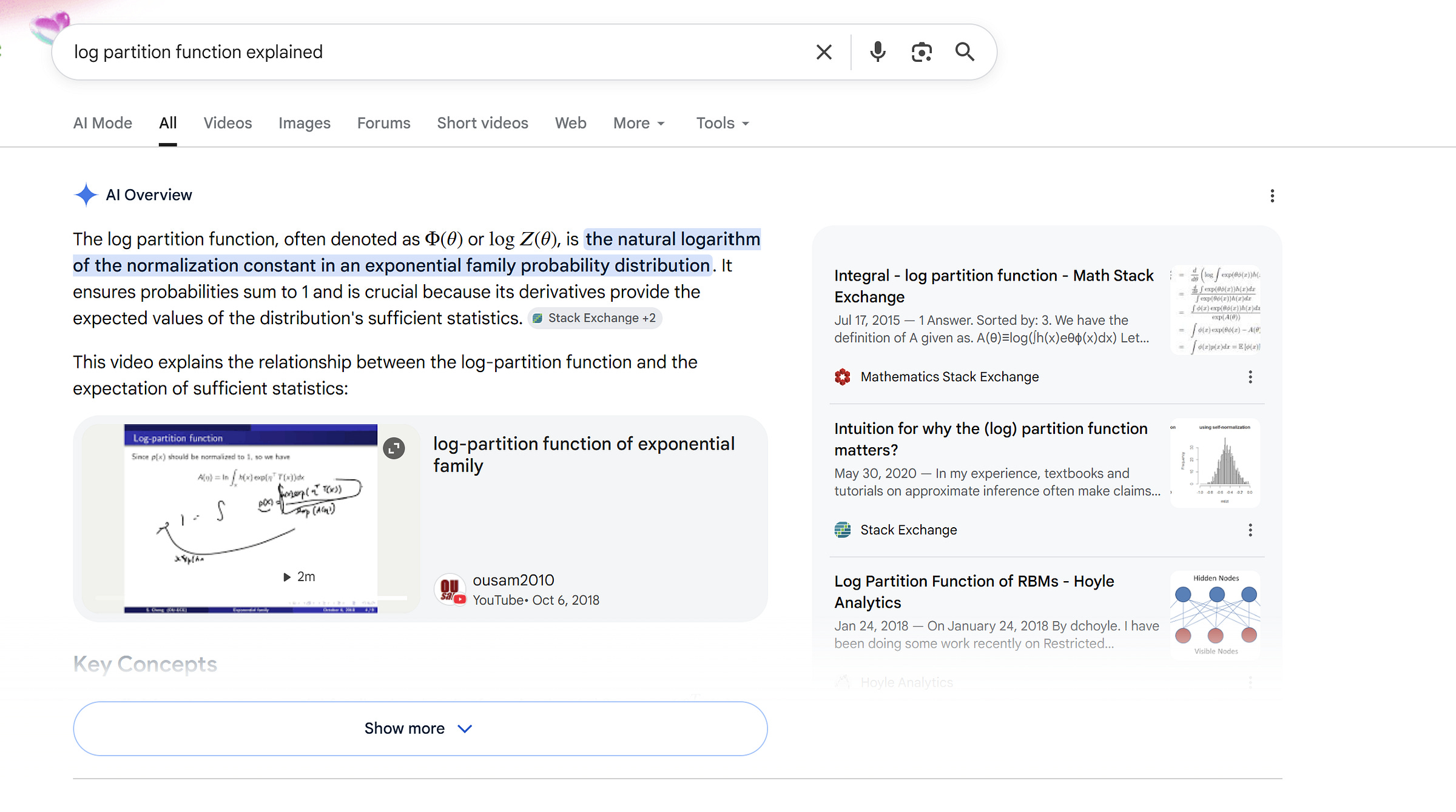
All of this chaos is controlled by the denominator in that Softmax equation — the normalizer that divides everything. Because we usually work in log-space to keep our GPUs from throwing underflow errors, we take the log of that massive sum. This term is so fundamental it gets its own name: the log-partition function, written as A(lambda).
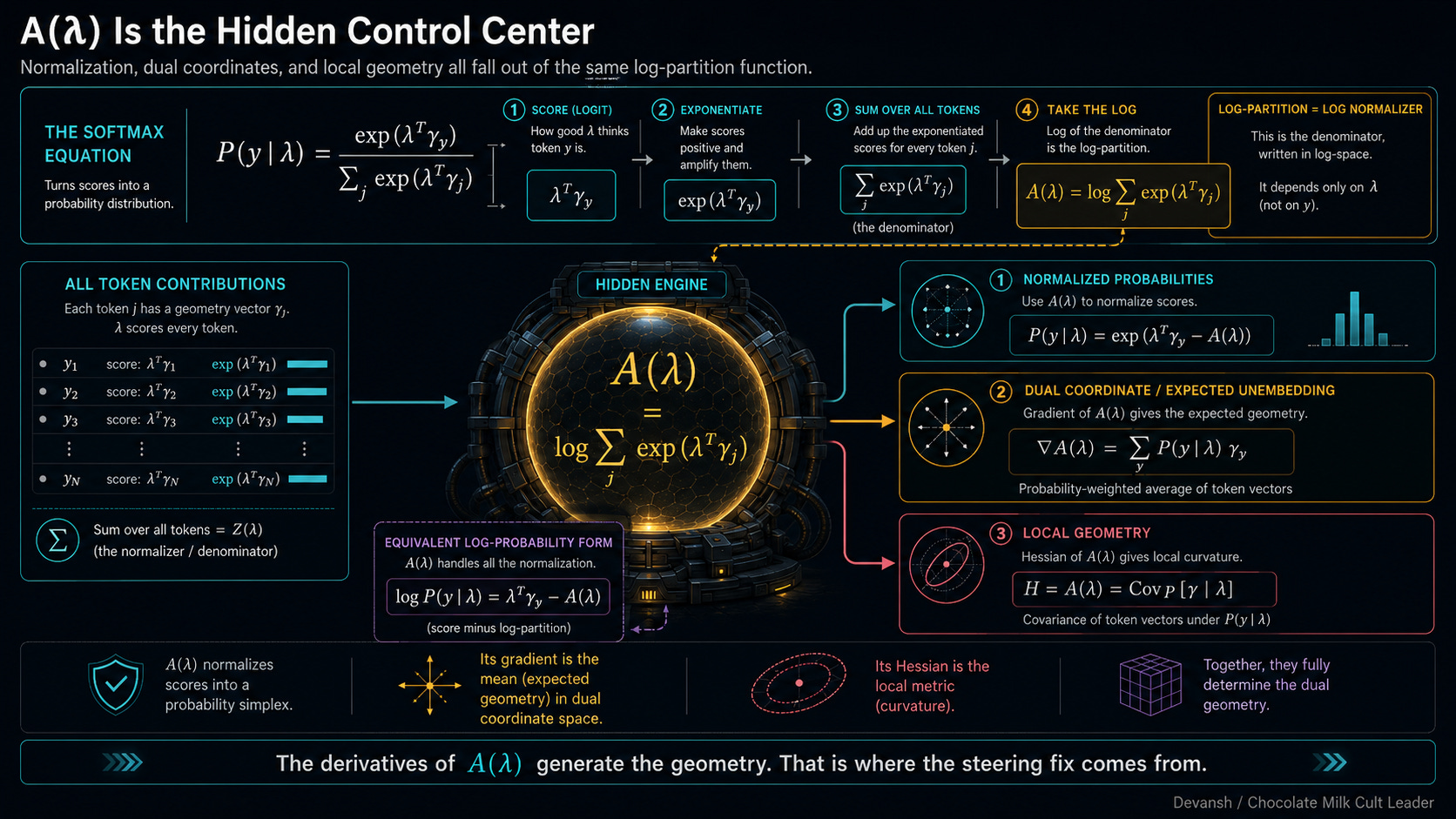
The actual probability of a token is just its exponentiated score minus this A(lambda) function. A handles all the normalization. This creates a very interesting outcome: the geometry of this space, the duality we need, and the steering fix we are about to build — all of it is hiding inside the derivatives of A(lambda).
To see why, we need a way to measure how different two softmax distributions are. And that leads us to our next point of exploration…
Why Does KL Divergence Measure the Change We Actually Care About?
We just established that the log-partition function A(lambda) controls the shape of our representation space. But before we can use it to fix our steering vectors, we have to solve a more immediate problem: how do we measure distance on this new terrain?
If Euclidean distance is a lie (yet another reason to not trust the Greeks)— if it treats a massive shove at 99% confidence exactly the same as a tiny nudge at a decision boundary — then what is the truth? We need a function that takes two probability distributions, compares them, and returns a single number representing how different they actually are in practice.
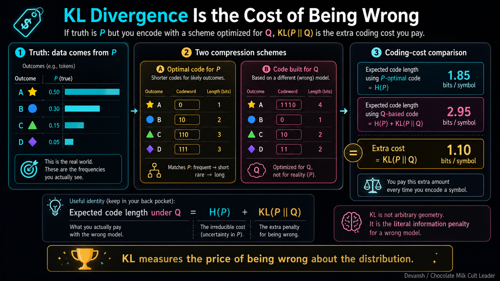
Our hero comes from Information Theoery: Kullback-Leibler (KL) divergence. If the true distribution is P, but your model assumes the distribution is Q, KL(P || Q) is the exact mathematical cost of that error. It calculates how surprised you will be when reality actually happens.
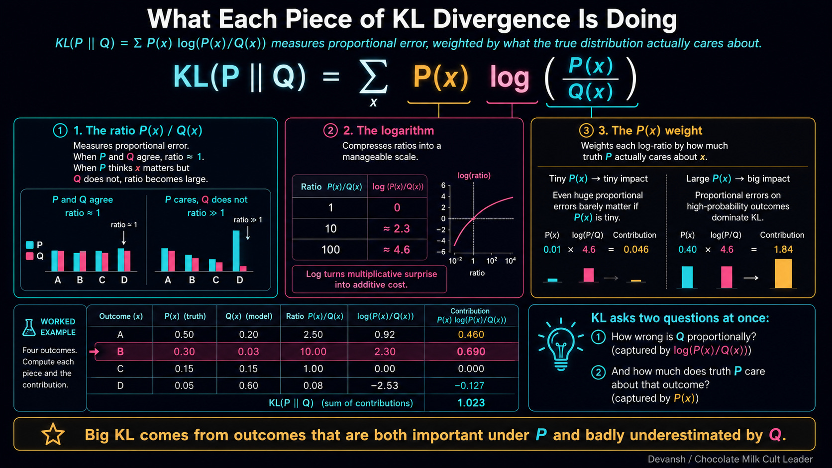
The formula is a sum over all possible outcomes x: P(x) * log(P(x) / Q(x)).
There are three moving parts here, and they each do a specific job to keep the math grounded in reality:
1. The Ratio: P(x) / Q(x) For any token x, how much more likely is it under the true distribution (P) than your steered distribution (Q)? If they agree, the ratio is 1. If P thinks the token is a sure thing and Q thinks it’s impossible, the ratio explodes.
2. The Logarithm Log converts multiplicative ratios into additive scores. A ratio of 1 (total agreement) maps to exactly zero. But more importantly, log makes KL sensitive to proportional changes, not absolute ones. A token dropping from 50% to 40% is only a 1.25x change. A token dropping from 0.1% to 0.01% is a 10x change. Log mathematically enforces the rule that relative probability determines model behavior.
3. The Weighting: P(x) The whole thing is multiplied by P(x) before summing. This is the “Do I actually care?” filter. KL only punishes disagreements where the true distribution P actually puts probability mass. If P thinks a token is garbage (P(x) is near 0), that term vanishes. What about Qs thoughts? Respectfully, who gives us a fuck what a grunt like Q thinks when a baller like P has already made up its mind.
Putting everything together, KL(P || Q) asks: “If P is the absolute truth, how surprised would you be if you had to navigate the world using Q?”
This weighting creates a profound asymmetry. KL(P || Q) does not equal KL(Q || P). Being wrong about P when Q is true costs a different amount than being wrong about Q when P is true. In the Euclidean space, the distance from New York to London is the same as London to New York. In information space, the penalty depends entirely on which distribution is actually generating your data. This asymmetry is exactly what causes forward and reverse KL to produce entirely different behaviors (which becomes the crucial AND-vs-OR distinction when we talk about interpolation later).
Why does this matter? Let’s dig into this math just a wee bit more. If we do this step-by-step, the geometry of the entire model falls out of the algebra.
What Happens When You Compute KL Between Two Softmax Distributions?
First, let’s put the pieces back on the board so we don’t lose track of what we are building:
lambda is our original, unsteered context vector.
lambda-prime is the steered vector (after we add our behavioral tweak).
gamma_y is the unembedding vector for a specific token (the dictionary definition the model checks against).
A(lambda) is the log-partition function — the brutal normalizer that forces everything to sum to 100%.
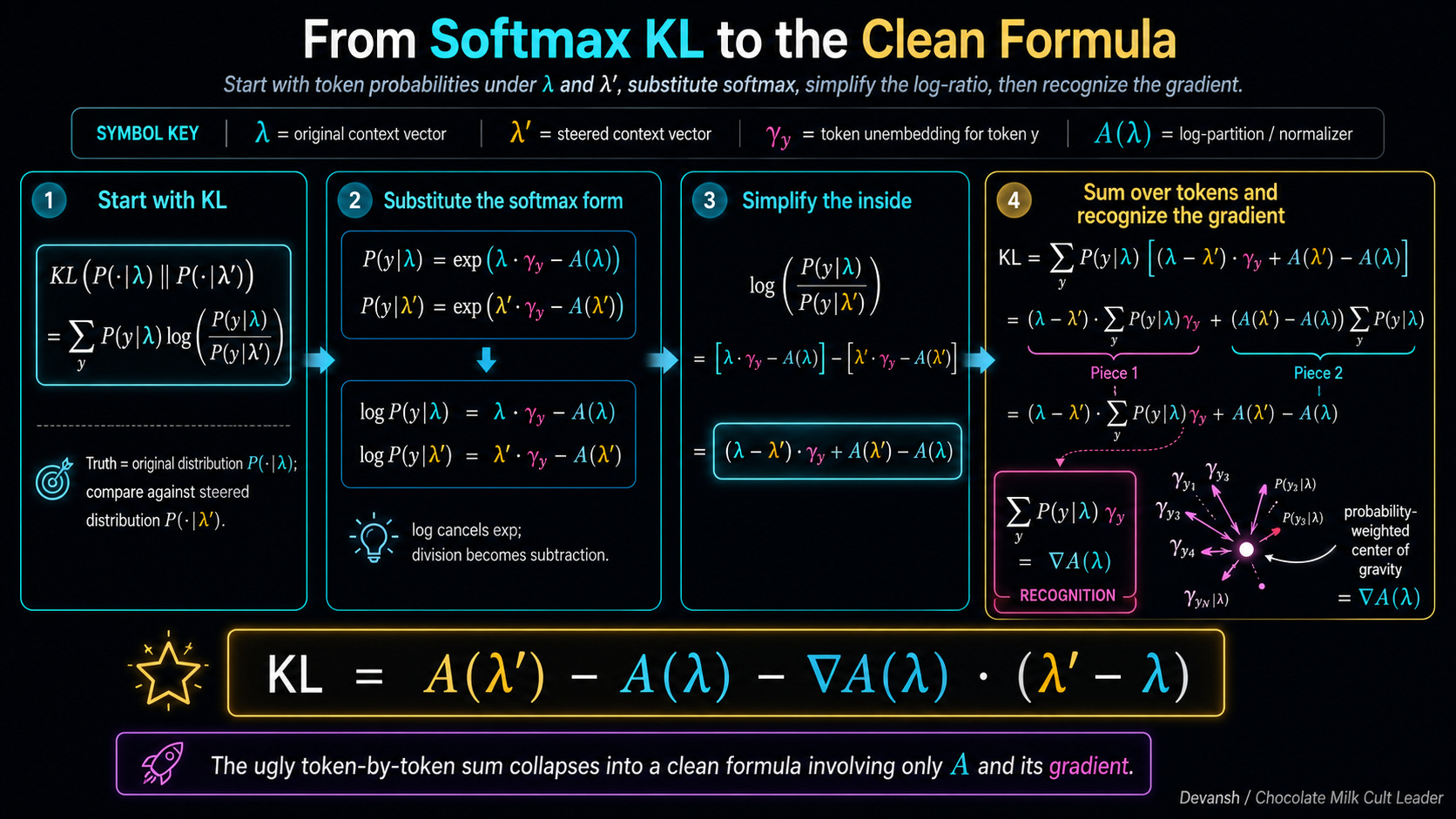
The KL formula asks us to compute a ratio for every token: log [ P(y | lambda) / P(y | lambda-prime) ].
In plain English: take the logarithm of the true probability divided by the steered probability.
How do we calculate those probabilities? Remember from the previous section: the probability of a token is just exp(score - normalizer).
Because we are taking the logarithm of an exponentiated number, the math simplifies beautifully. The log simply deletes the exp, leaving only the raw terms inside. Division inside a logarithm becomes subtraction outside.
So, taking the log of that probability ratio strips the math down to just the raw scores and the normalizers. For the top part of the fraction (the original state), we get: lambda * gamma_y - A(lambda)
For the bottom part (the steered state), we subtract it: minus [ lambda-prime * gamma_y - A(lambda-prime) ]
If you group the similar terms together, the log ratio becomes a clean, linear equation:
(lambda - lambda-prime) * gamma_y + A(lambda-prime) - A(lambda)
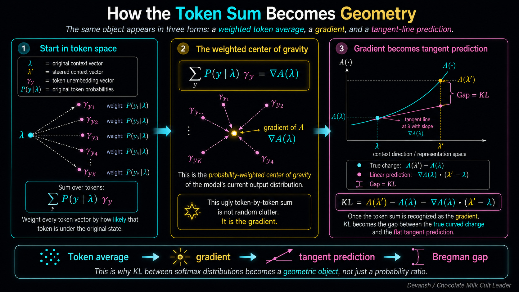
Now, the final step of the KL divergence formula tells us to multiply that result by the true probability P(y | lambda) and sum it up over every token in the vocabulary.
When you do that, something fascinating happens to that gamma_y term. You end up calculating the sum of P(y | lambda) * gamma_y.
Stop and think about what that is physically. You are taking every single token vector in the model, weighting it by how likely that token is to be generated, and averaging them all together. It is the probability-weighted center of gravity for the model’s current state.
As it turns out (and we will prove exactly why in the next section), this center of gravity is exactly the mathematical gradient of our log-partition function A. Let’s just call it grad-A(lambda).
If we substitute that gradient back into our equation, the final KL formula reveals itself:
KL = A(lambda-prime) - A(lambda) - grad-A(lambda) * (lambda-prime - lambda)
Look at the physical architecture of this final result.
A(lambda-prime) - A(lambda) is exactly how much the normalizer actually changed when we steered the vector.
grad-A(lambda) * (lambda-prime - lambda) is how much a straight, flat tangent line predicted the normalizer would change.
The KL divergence is literally the gap between the true change and the linear approximation.

Why is this gap always positive? Because the normalizer function A is convex — it curves upward like a bowl. For any convex function, a straight tangent line will always sit below the curve. The true curve always bends up and overshoots the straight-line prediction. The gap only hits zero if the two vectors are exactly the same.
This gap — the error between a convex function and its linear approximation — has a formal mathematical name. It is a Bregman divergence.
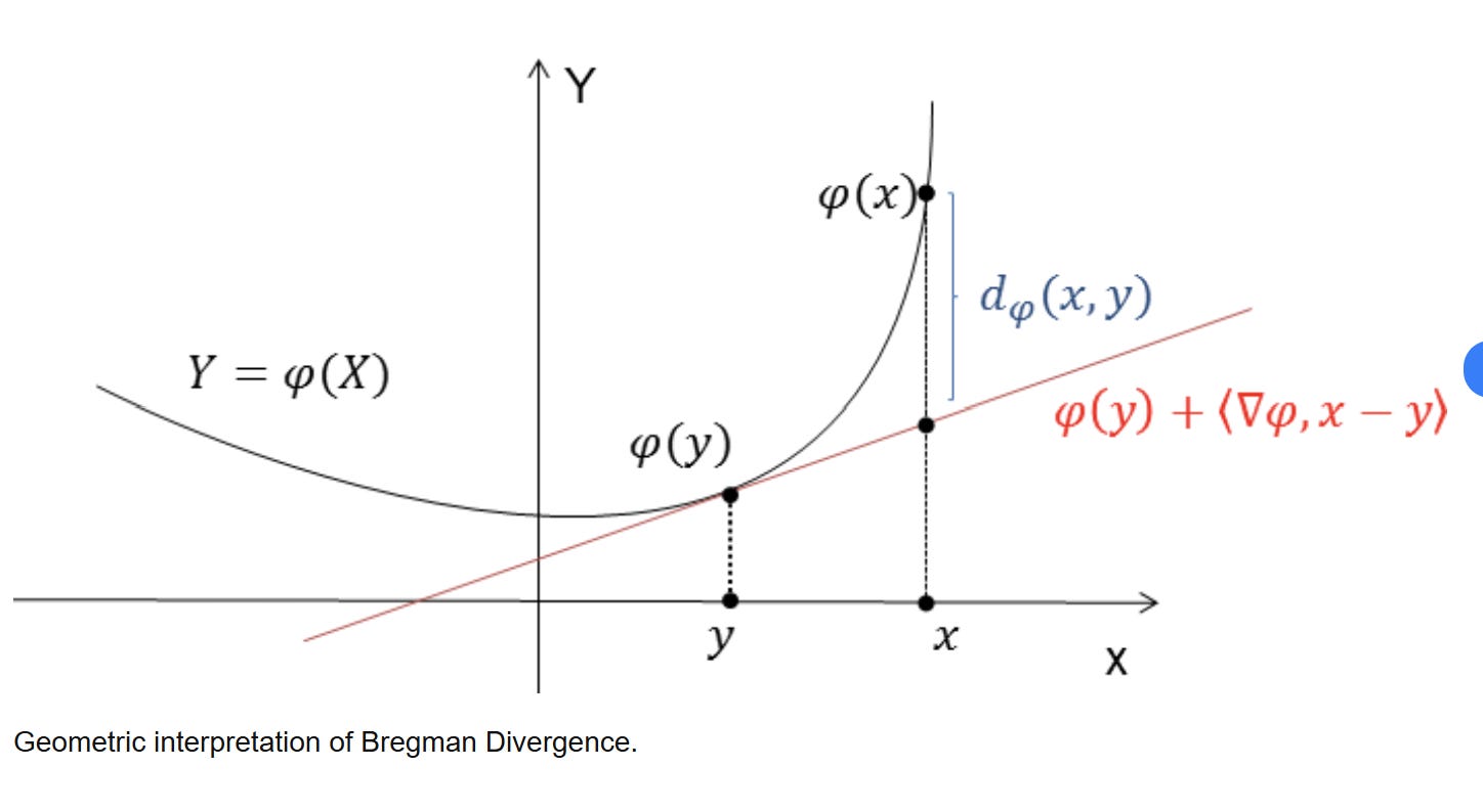
KL(P || Q) between two softmax distributions isn’t like a Bregman divergence. It is the Bregman divergence induced by the log-partition function A.
Nobody chose this. The algebra forced it. It means Euclidean geometry is not the natural default once a representation passes through a Softmax distribution. Every LLM, every CLIP model, and every attention layer is living and breathing in a Bregman geometry that most researchers have never explicitly mapped out. We’ve been using Euclidean wrenches on Bregman bolts since 2017.
Information geometers have studied Bregman divergences since the 1980s. And the very first thing their toolkit tells you about a space governed by Bregman geometry is this: the representation space does not have one natural coordinate system. It has two. This has some very juicy implications.
What Are the Two Coordinate Systems, and Why Does the Duality Matter?
The first coordinate system is the one everyone already uses: lambda. This is the raw representation vector sitting in the residual stream. Let’s call it the primal coordinate.
The primal space is the Wild West. It is entirely unconstrained. You can take your lambda vector, multiply it by a million, and point it absolutely anywhere in that 4,096-dimensional space. The model won’t crash. Softmax will just take those massive numbers and turn the output into a brutal step-function where one token gets 99.999% of the mass. The Primal Space has that good ol’ Murican freedom, baby.
The second coordinate system is completely different. It comes directly from that gradient term we isolated earlier: the gradient of our log-partition function. Let’s call this new coordinate phi.
phi = grad-A(lambda)
Let’s walk through the actual derivative (in case you don’t remember, derivatives give us the rate of change of something with respect to something else) to see what phi is physically made of. Don’t skip this, because it is the most elegant piece of math in the entire architecture.
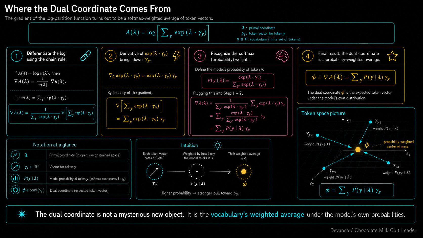
Remember that our normalizer function is A(lambda) = log [ sum of all exp(scores) ].
To find the gradient, we take the derivative. The chain rule in calculus tells us that the derivative of a logarithm is simply 1 / x multiplied by the derivative of whatever is inside the log.
The bottom of our fraction (the
x) becomes the inside of the log: the sum of all the exponentiated scores.The top of our fraction becomes the derivative of those scores. If a token’s score is
lambda * gamma_y, its derivative with respect to lambda is just the token vector itself:gamma_y.
So, for any given token, the gradient gives us this exact fraction: exp(score) / [sum of all exp(scores)] ... multiplied by the token vector gamma_y.
Look very closely at the left side of that multiplication. That fraction is literally the exact formula for Softmax probability.
The algebra just handed us a massive gift. The gradient of the log-partition function is simply every single token vector in the model, multiplied by its Softmax probability, and added together.
phi = sum over y of [ P(y | lambda) * gamma_y ]
This is our dual coordinate. Physically, it is the probability-weighted center of mass for the entire vocabulary. If the model assigns 70% probability to “maintains”, 20% to “operates”, and 10% to random noise, then your dual coordinate (phi) sits exactly at 0.7 * (maintains) + 0.2 * (operates) + 0.1 * (noise). It is a physical coordinate telling you exactly where the model’s attention is currently hovering across the dictionary.
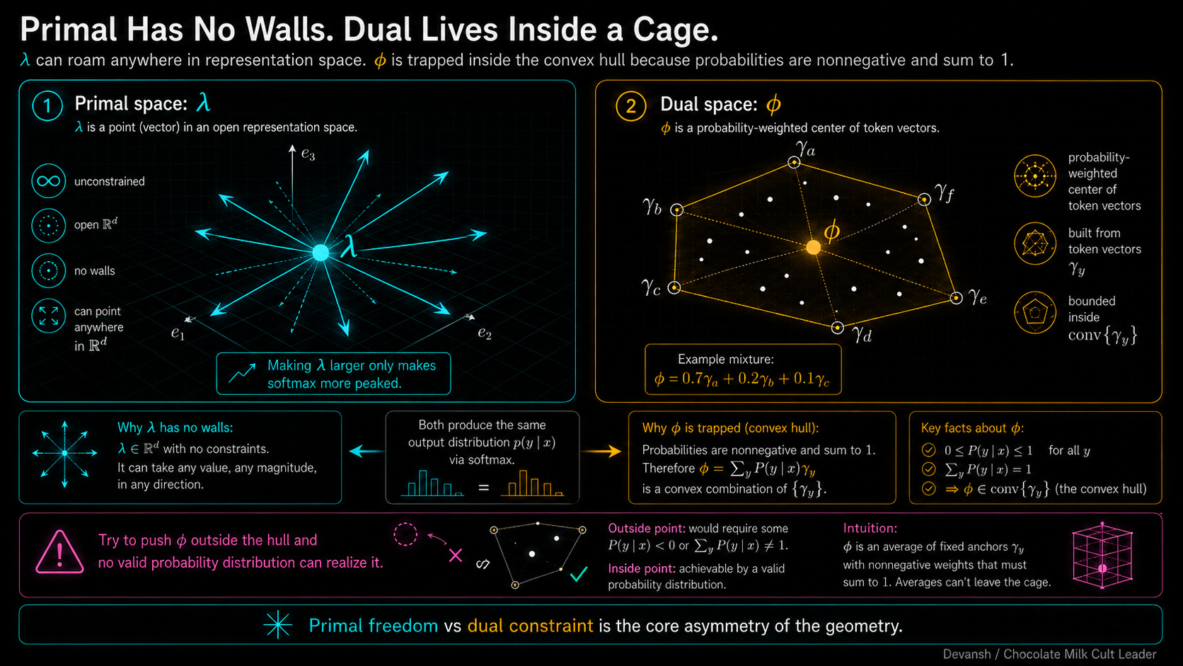
Because of how Bregman geometry works, lambda and phi are just two views of the exact same distribution. If you have the primal vector, you can calculate the dual center of mass. If you have the dual center of mass, you can reverse-engineer the primal vector.
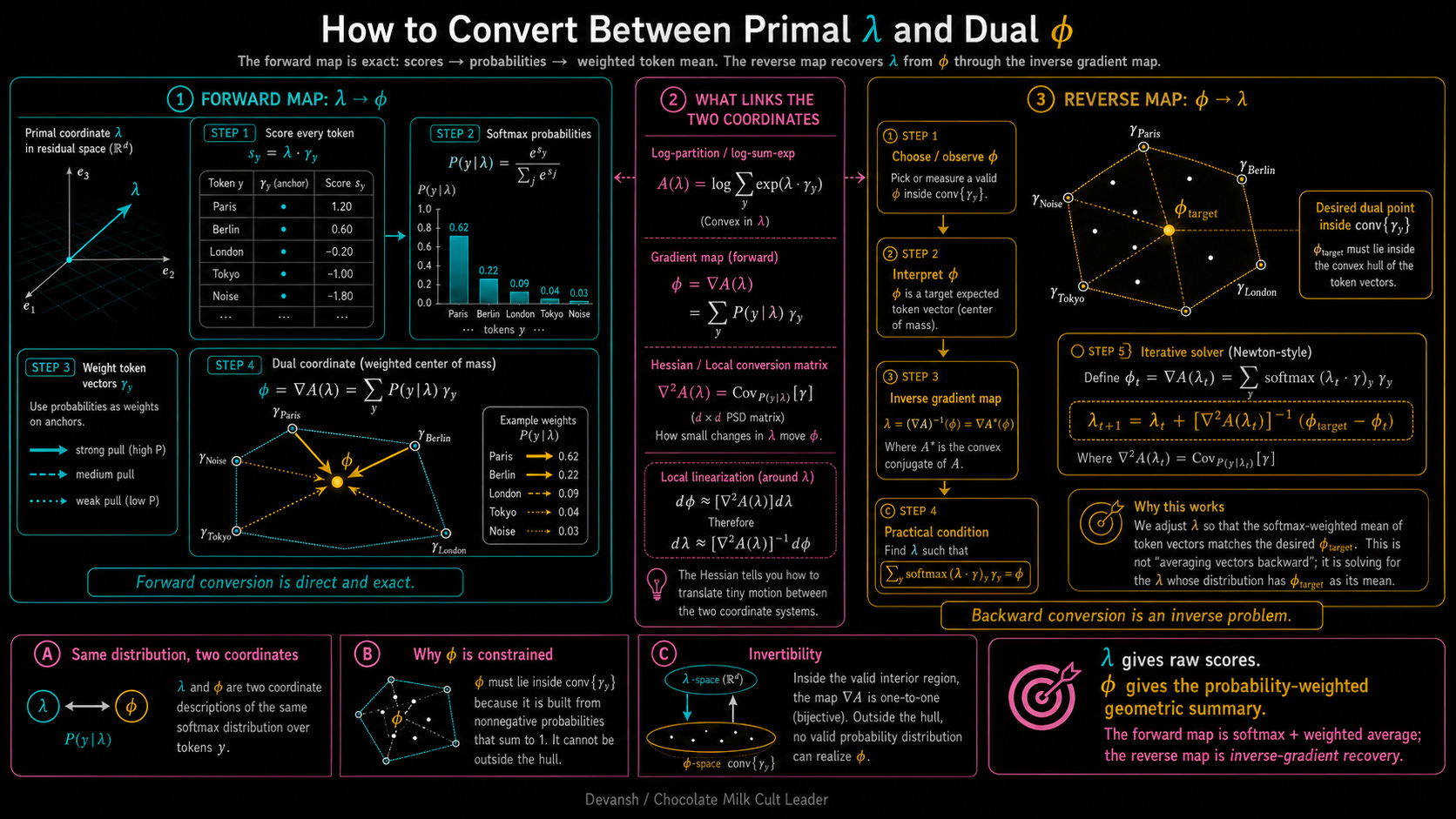
But there is a massive physical asymmetry between them. We already established that the primal space (lambda) is infinite. The dual space (phi) is trapped in a cage.
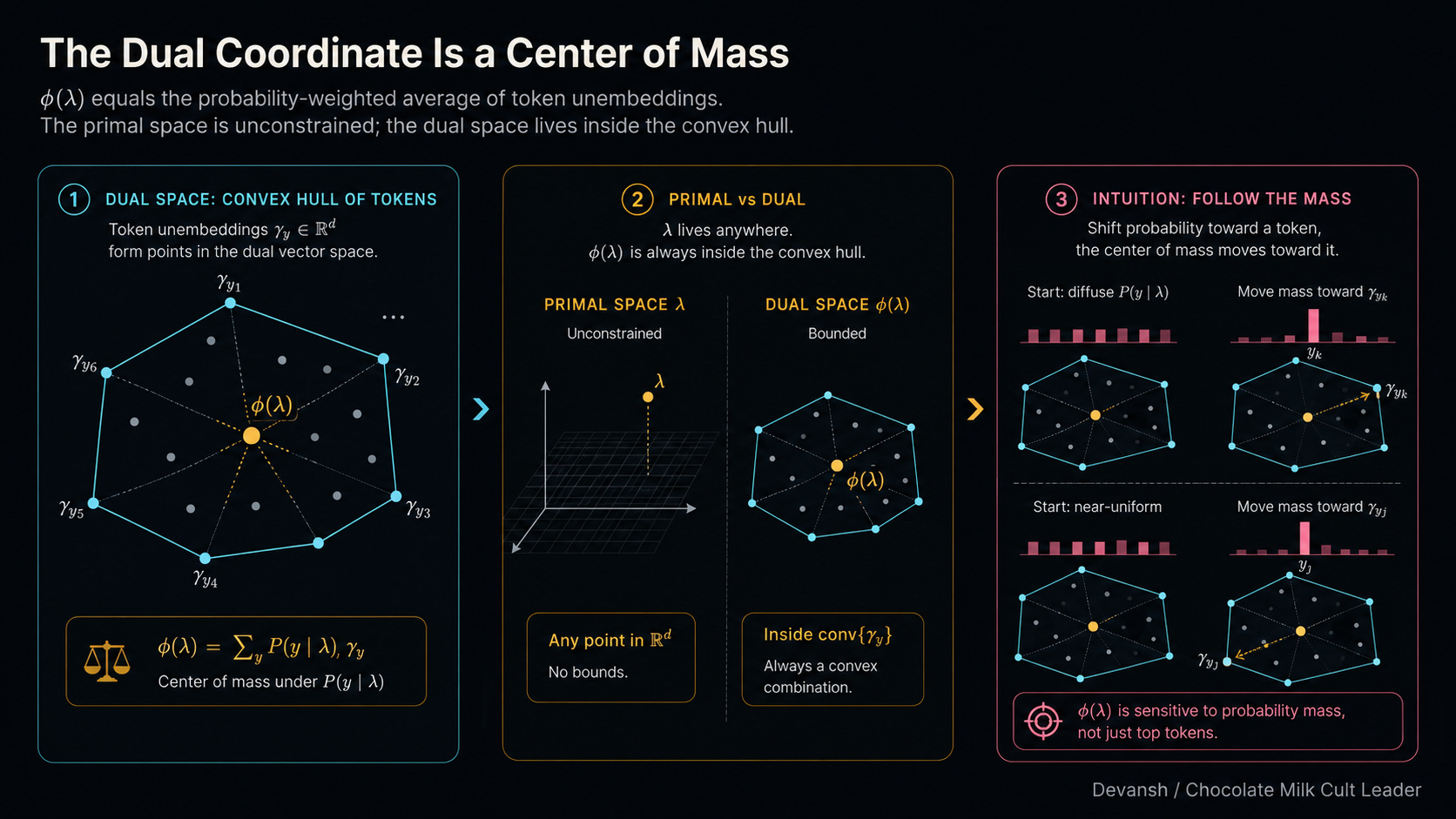
Why? Because phi is built by multiplying token vectors by probabilities. Probabilities obey strict laws: they can never be negative, and they must add up to exactly 100%. Because of this, phi can never step outside the boundary drawn around your vocabulary. Imagine stretching a massive mathematical rubber band around every single token vector in the model’s embedding space. That rubber band is called a convex hull. You can move phi anywhere inside the hull by mixing different token probabilities, but you can never push it outside. If you try to steer the dual coordinate outside that hull, the math shatters, because no valid probability distribution could ever put you there.
What Do the Two Coordinate Systems Mean Semantically?
Why do we care that there are two systems? Because they answer the most basic question in geometry completely differently: how do you draw a straight line? This might seem like a silly questions, but drawing a straight line between two concepts is how we blend them. When you want to combine two ideas, you take their representations and find the midpoint. But on a warped Bregman surface, your midpoint completely depends on which coordinate system you use to draw the line.
Let’s look at a concrete example. You have two representations.
Vector 0 is the model’s state after reading: “Q: What is the capital of France? A: It is” (Probability sits heavily on the token “Paris”).
Vector 1 is the state after reading: “Q: What is the capital of Germany? A: It is” (Probability sits heavily on “Berlin”).
You want to find the exact 50/50 midpoint between these two concepts.
If you do a primal interpolation, you draw a straight line between the two raw lambda vectors in the unconstrained residual stream. Because of how the Bregman algebra shakes out, moving in a straight line in primal space mathematically forces the model to minimize the reverse KL divergence.
Think back to our KL section. Reverse KL is the “Do Not Hallucinate” penalty. It looks at the target distribution and says, “If the target thinks a token is garbage, you will pay a massive penalty for putting probability mass there.”
Look at what happens to the math when you stand at the primal midpoint. The France endpoint looks at the word “Berlin.” It sees that “Berlin” has near-zero probability in the France distribution, so it slaps the model with a massive penalty for including it. Simultaneously, the Germany endpoint looks at the word “Paris,” sees near-zero probability, and slaps the model with a massive penalty for including it.
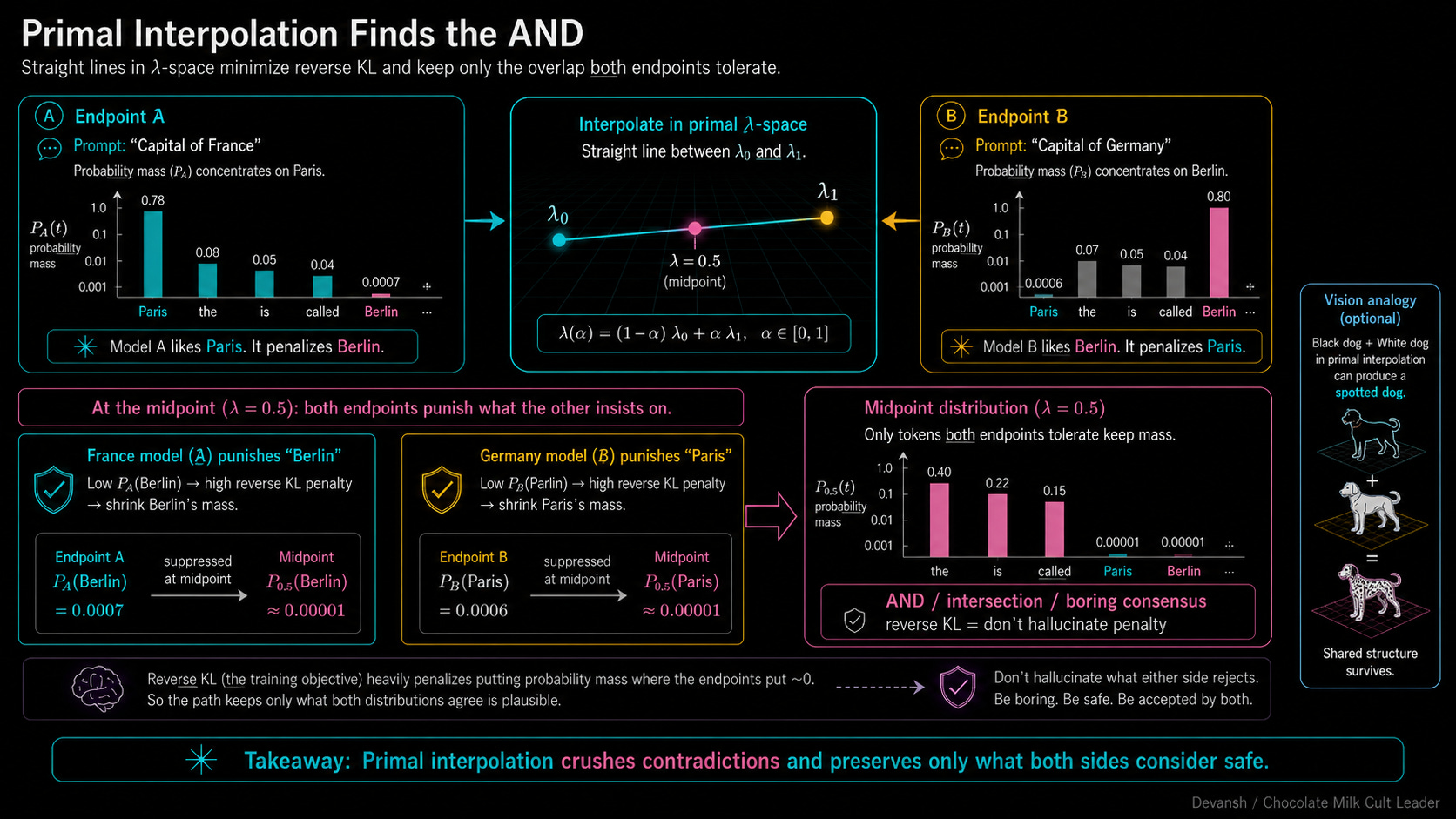
What survives? Only the tokens that both endpoints agree are mathematically harmless — generic words like “The”, “is”, or “called”. Primal interpolation operates exactly like a logical AND. It crushes everything that makes a context unique and leaves only the safest possible intersection.
If you do a dual interpolation, you draw a straight line between the two phi vectors (the centers of mass) inside the convex hull. Moving in a straight line in dual space minimizes the forward KL divergence.
Forward KL operates under the exact opposite philosophy. It is the “Do Not Forget” penalty. It says, “If the target thinks a token is highly likely, you will pay a massive penalty if you fail to cover it.”
Look at the midpoint now. The endpoints are no longer allowed to veto each other. France demands you keep “Paris”. Germany demands you keep “Berlin”. Instead of crushing them, dual interpolation forces the model into a compromise. It creates a mixed probability distribution that holds both truths simultaneously, allocating roughly 50% mass to Paris and 50% mass to Berlin.
In other words, Dual interpolation operates exactly like a logical OR. It preserves the union of the two concepts.
This behavior is a fundamental law of any model that uses Softmax. If you take a vision model like CLIP and try to interpolate the concept of a “black dog” with a “white dog”, you get the exact same split.
Primal interpolation (AND logic) searches for shared traits. The colors fight each other, the model panics, and it spits out a single dog with black and white spots.
Dual interpolation (OR logic) holds both truths. It spits out an image that literally contains two distinct dogs — one black, one white.
Primal finds the boring consensus. Dual preserves the contradiction. Two completely different philosophies of blending concepts, arising purely from which ruler you picked up.
This is why the geometry actually matters for your pipeline. When you blindly subtract two vectors in the residual stream to build a steering direction, you aren’t just doing niche math. You are accidentally making a product decision. By calculating your vector in the raw residual stream, you are locking yourself into the primal coordinate system. You are forcing the model into that destructive AND logic. You are explicitly telling the model to crush anything unique about the prompt and only keep the safe consensus. This is exactly why standard steering leaks probability mass to generic prepositions like “to” — it’s abandoning specific concepts to find the mathematical middle ground.
If you actually want to add a behavioral concept without destroying the original context — if you want the OR logic — you cannot just add vectors in the residual stream. You have to translate the vectors, do the addition in the dual space, and translate them back.
Isn’t exploring the math of intelligence so much cooler than being a training grunt? Imagine learning about some of the coolest topics in the world only to be forced to debug GPU crashes and benchmark tests 24/7.
Interpolation shows that the two coordinate systems produce different behaviors when you blend representations. Steering is a related but sharper operation: instead of blending two representations, you’re modifying one to change a specific concept. The question is the same — which coordinate system are you operating in? — but the stakes are higher, because steering with a probe means adding a specific mathematical object to the representation. What kind of object the probe is determines which coordinate system it belongs to.
What Kind of Mathematical Object Is a Linear Probe?
Before we fix the steering math, we have to look closely at the tool we are using to steer: the linear probe.
When you train a linear probe to detect a concept — say, “third-person verb” — you are building a very specific mathematical object. It takes your 4,096-dimensional representation vector (lambda), runs a dot product against its own weights (beta_W), and spits out a single scalar score.
In linear algebra, an object that eats vectors and spits out scalars is a linear functional. A covector. Covectors live exclusively in the dual space.
Most of us learned the difference between vectors and covectors in undergrad and immediately dumped it from RAM. Why? Because if you live in flat Euclidean space, you don’t need to care. Flat space lets you cheat. You can add them, subtract them, and treat a covector exactly like a normal vector.
But they are physically different objects.
A vector is a displacement — a physical direction you can move. A covector is a measurement — a tool that assigns numbers to states. Think of a thermometer. A thermometer measures a room and returns a temperature. The thermometer itself is not a room. You cannot take a physical location and mathematically “add” a thermometer to it.
In the warped, twisted Bregman geometry of Neural Network Information Spaces, we can’t get away with conflating them. Technically, we can, but that is why so much of the activation steering research has sucked for so long and all of the attention has been to the fine-tuning tards.
What Does Standard Activation Steering Get Horribly Wrong?
Look at the formula the entire open-source community currently uses for activation steering: lambda_t = lambda_0 + t * beta_W
Take the original context vector (lambda_0), add the probe (beta_W) multiplied by some steering strength (t).
As an array operation, it runs perfectly. PyTorch will execute the addition without throwing a warning because both objects are just float32 arrays of the same shape. But PyTorch doesn’t know geometry.
As a geometric operation, this equation is a disaster. It blindly mashes a measurement tool (the probe) into a physical displacement (the representation). Because Softmax forces the model into Bregman space, vectors and covectors are not interchangeable.
But Dev Dev, you can say it sucks, but I don’t understand why. What does this type of error cost you in production?
When standard steering executes that addition, it is mathematically asking the model to find the closest point that satisfies the new concept. But because it used Euclidean math, which we already proved has zero relationship to the model’s actual output distribution. Put two and two together and we see that — that gap (the distance between the Euclidean guess and the true Bregman reality ) is exactly where your probability leaks. It is the physical reason the preposition “to” steals all the mass from your verbs. It is the reason your vision model spits out a dog with black and white spots instead of two distinct dogs.
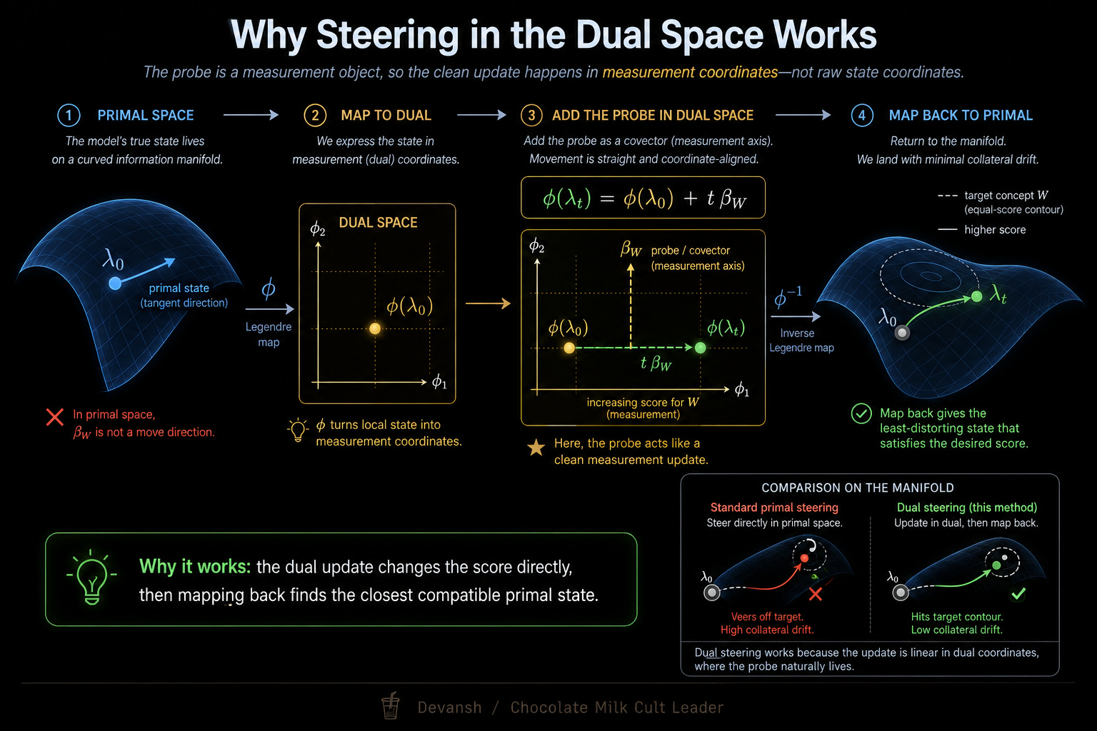
The fix is one line of math.
phi(lambda_t) = phi(lambda_0) + t * beta_W
Map your primal vector to the dual coordinate system (phi). Add the probe (beta_W) in the dual space, where measurement tools actually belong. Then translate the result back to primal space to hand off to the next layer.
So what does this actually accomplish? A lot, actually.
The Payoff: What Actually Happens in Production?
What happens to Gemma-3–4B?
The hallucination dies. When you run the dual steering vector to change a base verb to a third-person verb, the probability mass shifts directly from “maintain” to “maintains”. That generic preposition “to” that spiked out of nowhere in the primal space? It stays completely flat. The probability leak is sealed.
What happens to the vision models?
Steer MetaCLIP-2 away from “cat” toward “dog” in dual space, and the model directly transfers probability to images of dogs. The off-target “cat and dog sitting together” image never spikes.
Why Does Dual Steering Actually Work?
When you steer in the primal space, you are just adding raw numbers to the model’s logits. Softmax then exponentiates those inflated numbers. Because exponentiation amplifies differences, the artificially massive logits crush the model’s original context. To make everything sum to 100%, the model abandons the specific context and falls back on the safest, most frequent tokens it knows. As with most things in life, an overabundance of playing it safe leads to bland, generic output (tokens like to).
The dual space (phi) operates under different laws. Because it is built entirely from probabilities, it is strictly zero-sum. The total mass is locked at exactly 100%. You cannot inject raw, unconstrained numbers here.
If you want to push the center of mass toward the third-person verb “maintains”, the math forces a direct trade. This trade is the physical reality of a “KL projection.” The projection takes your target concept and solves for a new probability distribution using two strict rules: the new distribution must satisfy your steering target, and it must change the original probabilities as little as physically possible.
To satisfy both rules, it steals the required probability mass directly from the base verb (“maintain”) and hands it to the target verb (“maintains”). The generic token “to” stays flat because the distribution was never shattered.
That’s not to say this is without flaws. Dual steering fixes the geometric type error, but it hits a hard wall in production: it only works at the exit nodes.
The Bregman geometry derived by Park et al. relies entirely on the log-partition function. That means it only applies to representations passing directly through a Softmax distribution. In modern architectures, that restricts you to the final-token unembedding layer, CLIP retrievals, and attention matrices.
In production, almost nobody steers at the final layer. By the time a concept hits the unembedding matrix, the model has already made its decision. Surgical steering happens deep inside the network — say, layer 15 of a 32-layer model — to intercept a concept before it fully forms. But intermediate layers don’t have a Softmax attached to them. They are just unconstrained states floating in the residual stream. For intermediate layers, the mathematical map of Bregman geometry simply stops.
So…. we can never really apply the math we just talked about to hit real-time steering. That is a slight problem.
So where does this leave us? Do we just retard-max and let fine-tuning handle all the work? Let’s bring our little exploration to a close.
Conclusion: Where Does Dual Steering Go From Here.
Let’s end our journey with a trip down memory lane, back to the days of classic ML. Think about how LLMs changed production. We used to build massive, brittle scaffolding — wiring ten specialized ML classifiers to two generators just to complete one basic workflow. LLMs replaced all of that with a single general-purpose model, collapsing infrastructure costs overnight. That drop in cost didn’t happen because we optimized the classifiers. It happened because we completely changed the interaction pattern.

We are at the exact same threshold with model internals.
Right now, the industry’s default reflex for bad model behavior is to treat it as an infrastructure problem. When a model fails, we throw compute at it. We run brittle fine-tuning jobs and try to bludgeon the network into submission using scale.
But as more research is showing, the model layer might be the wrong layer to solve these problems. Perhaps the true solution is deeper. By changing how the space of how we represent knowledge in the language models, and then how we navigate it, we might be able to unlock capabilities that our current paradigm deems unrealistic.
And even if it doesn’t work, isn’t the idea so much more fun? Do you really want to spend the rest of your career profiling GPUs, fiddling with random seeds, and writing 20 skills/agent templates so that your manager can show your teams AI readiness? Does your heart (and brain) not ache to do more, to push humanity’s knowledge forward?
Think that over.
Thank you for being here, and I hope you have a wonderful day,
Dev <3
If you liked this article and wish to share it, please refer to the following guidelines.
That is it for this piece. I appreciate your time. As always, if you’re interested in working with me or checking out my other work, my links will be at the end of this email/post. And if you found value in this write-up, I would appreciate you sharing it with more people. It is word-of-mouth referrals like yours that help me grow. The best way to share testimonials is to share articles and tag me in your post so I can see/share it.

Reach out to me
Use the links below to check out my other content, learn more about tutoring, reach out to me about projects, or just to say hi.
Small Snippets about Tech, AI and Machine Learning over here
AI Newsletter- https://artificialintelligencemadesimple.substack.com/
My grandma’s favorite Tech Newsletter- https://codinginterviewsmadesimple.substack.com/
My (imaginary) sister’s favorite MLOps Podcast-
Check out my other articles on Medium. :
https://machine-learning-made-simple.medium.com/
My YouTube: https://www.youtube.com/@ChocolateMilkCultLeader/
Reach out to me on LinkedIn. Let’s connect: https://www.linkedin.com/in/devansh-devansh-516004168/
My Instagram: https://www.instagram.com/iseethings404/
My Twitter: https://twitter.com/Machine01776819
so.. fine tuning it is?
The strongest cult and community analysis usually comes from people willing to examine the emotional needs, loneliness, identity formation, and desire for belonging underneath the surface behavior.