How to Reduce the costs of Running LLMs by 10-15x [Investigations]

The Official Chocolate Milk Cult's Guide to Inference Scaling for AI Models

Sep 21, 2025

It takes time to create work that’s clear, independent, and genuinely useful. If you’ve found value in this newsletter, consider becoming a paid subscriber. It helps me dive deeper into research, reach more people, stay free from ads/hidden agendas, and supports my crippling chocolate milk addiction. We run on a “pay what you can” model—so if you believe in the mission, there’s likely a plan that fits (over here).

Every subscription helps me stay independent, avoid clickbait, and focus on depth over noise, and I deeply appreciate everyone who chooses to support our cult.

Help me buy chocolate milk

PS – Supporting this work doesn’t have to come out of your pocket. If you read this as part of your professional development, you can use this email template to request reimbursement for your subscription.

Every month, the Chocolate Milk Cult reaches over a million Builders, Investors, Policy Makers, Leaders, and more. If you’d like to meet other members of our community, please fill out this contact form here (I will never sell your data nor will I make intros w/o your explicit permission)- https://forms.gle/Pi1pGLuS1FmzXoLr6

Inference Scaling is one of the most hyped ideas in AI in the AI landscape right now. Nvidia, cloud hyper-scalers, and other infrastructure players are pivoting to inference scaling (relying on more AI inference calls to maximize the performance of AI systems) to avoid the diminishing returns from scaling up the model training. Anyone building AI Solutions (or investing in them) should be deeply familiar with the space as it is undeniably one of the biggest trends in the market.

“Test time scaling is going to go through the roof…especially with Agentic Systems and more capable models”
— Jensen Huang. Greg Brockman, Sundar Pichai, and others have pointed to something similar.

This article will give you a comprehensive list of the most powerful techniques to enable AI inference scaling. All techniques mentioned here have been tested at the Chocolate Milk Cult and deployed by our team for various clients and are used by the top AI Labs to improve the performance of their AI models w/o breaking the bank. However, since there are many ways to skin a cat, I want to establish your expectations upfront. Here are a few classes of techniques that will NOT be covered —

Design-based Scaling: involves using smaller LLMs, Agents, Context Management, etc, to keep costs low. In my opinion, this is the best set of techniques to know, but it’s a whole different discussion. AI Engineering is 90% Software Engineering in most use-cases, and using design to scale natively is a key skill to pick up.
Model-Based Scaling: Trying things like Complex Valued NNs, Sparse Weight Activation Training, Coconut, Byte Latent Transformers, RWKV etc (all of which I think are very promising) all require training models ground up, which makes it impractical for most of us gareeb log.

In other words, we’re going to focus our attention squarely on techniques where you can take existing models and rework them using these various techniques. In a similar spirit, I’m also not going to focus on the absolutest powerful techniques, but keep my focus on things that I know most people can build around. The upper limit potential of a technique is useless if your 3 chichora team has to drop a milly on specialized AI Talent.

Disclaimer before the dumb ones jump in: these moves look simple. They’re not. You’ll choke on batching, parallel inference, hyper-parameter-fuckery, and the other nonsense from the wonderful world of ML Engineering. If your insane clown posse can’t handle that, stick with OpenAI/Gemini API and stop pretending you’re DeepMind.

Read this to help you get a handle for how much you might end up paying to use Open LLMs.

Executive Highlights (TL;DR of the Article)

There are 3 tiers to inference scaling, ordered by most to least important.

Tier 1 — Maximize Hardware Utilization

Keep the GPU fully busy; squeeze value from every cycle.

Batching & Parallelism: Continuous batching, prefill/decode split, and length-aware bucketing prevent idle cores and wasted compute on padding.
Compiler & Graph Execution: Kernel fusion, CUDA graphs, and FlashAttention cut memory traffic, reduce CPU overhead, and unlock long-context speedups.
Quantization: INT8/INT4 weight storage or FP8 math shrinks memory footprint; cheaper, faster, same quality when calibrated correctly.

Exit: ≥75% utilization, CUDA graphs in decode loop, quantized models with <1% quality loss.

Tier 2 — Algorithmic & Memory Warfare

Shift from FLOPs to bandwidth; reduce the memory choke points.

KV Cache Optimization: Paged KV, prefix reuse, MQA/GQA, KV quantization, and sliding window/forgetful attention keep memory from ballooning beyond 100k+ contexts.

Sparse Architectures:

MoE (parameter sparsity): trillion-scale capacity with conditional compute, but unstable without strong interconnects.
Sparse Attention (activation sparsity): restricts attention patterns to linearize cost.

Speculative Decoding: Pair a small draft model with the main LLM; verify predictions to cut passes and halve costs. We will also be talking about Medusa and Lookahead decoding as modern variants of Spec Decoding to address the draft model dependency.

Exit: Cache reuse visible, speculative decoding ≥2× speedup, sparse methods stable, 32k+ contexts running smoothly.

Tier 3 — The Marginal Gains

Kill death-by-a-thousand-cuts at scale.

Constrained Decoding: Mask invalid outputs (JSON, regex, tries) → higher correctness, shorter outputs, lower cost.
Distillation & Pruning: Shrink bloated models via logit distillation, structured pruning, or enforced sparsity (2:4) → 30–50% cheaper per token.
Verifiers: Reward/scoring models prune, stop, or redirect generations; powerful for agentic/legal use-cases.
Topology: Placement matters — model/data co-location, NUMA awareness, replicas vs. shards, response caching.
Policy Tuning: Sequence length is cost; tune sampling to trim 10–20% tokens.

Exit: Invalid outputs <0.1%, compressed models cheaper, cache hit rates ≥25%, tail latency stable, average tokens per output reduced.

The Bigger Question — Scaling for Whom?

Hyperscalers profit from endless scaling; each token deepens lock-in.
Builders gain cheaper inference and wider access — but risk reinforcing centralization.
History shows progress empowers individuals and entrenches elites; the treadmill expands capability but also chains.

The open challenge: how do we thrive and build in a world with scaling (which is coming anyway) while also ensuring a future where we’re not beholden to the ones that provide it to us?

I put a lot of work into writing this newsletter. To do so, I rely on you for support. If a few more people choose to become paid subscribers, the Chocolate Milk Cult can continue to provide high-quality and accessible education and opportunities to anyone who needs it. If you think this mission is worth contributing to, please consider a premium subscription. You can do so for less than the cost of a Netflix Subscription (pay what you want here).

I provide various consulting and advisory services. If you‘d like to explore how we can work together, reach out to me through any of my socials over here or reply to this email.

Tier 1 — Maximizing Hardware Utilization

A transformer is a giant calculator. Your GPU is the factory floor. If the floor is empty, no amount of clever math saves you. Tier 1 is about keeping every core busy, every cycle productive. You paid Nvidia a lot of money for your expensive sand, so it’s only right that you make sure that you beat it till it can’t stand anymore.

1.1 Batching & Parallelism for Efficient Inference

“Anthropic’s Claude 3 was optimized with continuous batching, boosting throughput from 50 to 450 tokens/second and significantly reducing latency (from ~2.5s to sub-second). Similarly, Anyscale reported that using continuous batching (along with memory optimizations) enabled up to 23× more throughput in LLM inference compared to naive per-request processing.” — Source (

Rohan Paul

is an excellent resource, highly recommend following him )

Batch inference in Large Language Models (LLMs) is a processing approach that groups multiple requests together for simultaneous execution. This method significantly improves computational efficiency and resource utilization compared to processing individual requests sequentially.

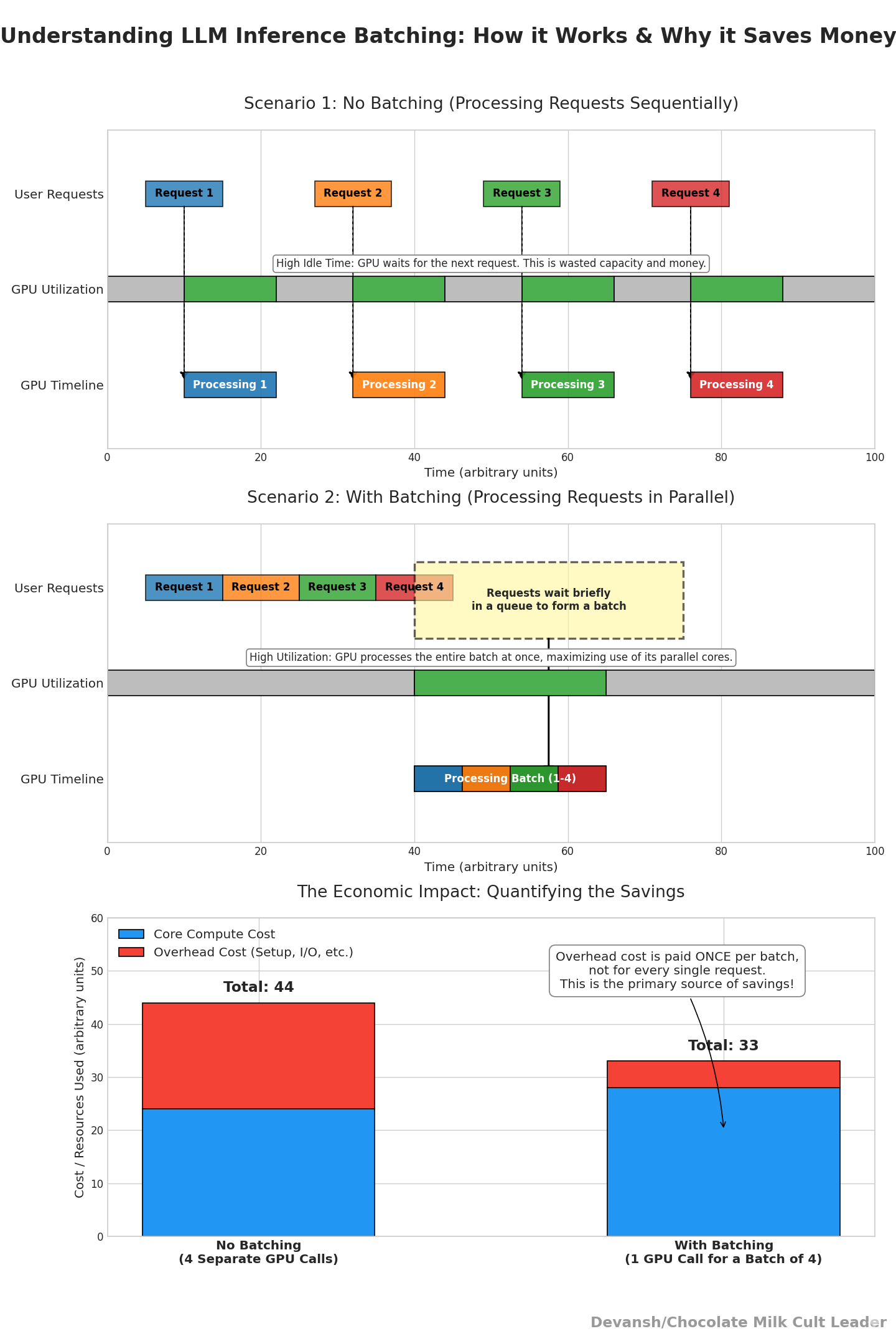
Understanding batching for LLM inference, how it works, and why cuts costs.

To understand how to leverage batching for peak performance, we must first take some time to understand the LLM inference process. Under the hood, your model.call() isn’t one thing. Instead, your LLM does two distinct things:

Prefill. It processes the entire input prompt at once. This is matrix multiplication heavy — exactly what GPUs are good at. More sequences in parallel = higher utilization.
Decode. It generates one token at a time. Each new token depends on the entire history of prior tokens. This phase is dominated by memory reads/writes rather than raw math.

If you treat prefill and decode the same, you either underutilize compute (during prefill) or blow up latency (during decode).

Now that you have the base understanding, you’ll be in a much better position to implement the following techniques to help you improve batching performance —

Continuous batching: Continuous batching uses iteration-level scheduling. At every single token generation step, the system checks if any sequence in the batch has completed. If one has, its resources are immediately freed, and a new request from the waiting queue is inserted into its slot for the very next iteration. This ensures the GPU remains perpetually saturated with active computations, leading to dramatic throughput improvements. (PS- Without Paged Attention, the constant adding and removing of sequences would lead to severe memory fragmentation, negating the benefits.)

With iteration-level scheduling, a next request will be scheduled as soon as a request finishes its iteration.

Prefill/Decode split: Prefill can be batched to a maximum size; decode should use small, responsive batches. Systems like vLLM formalize this split.
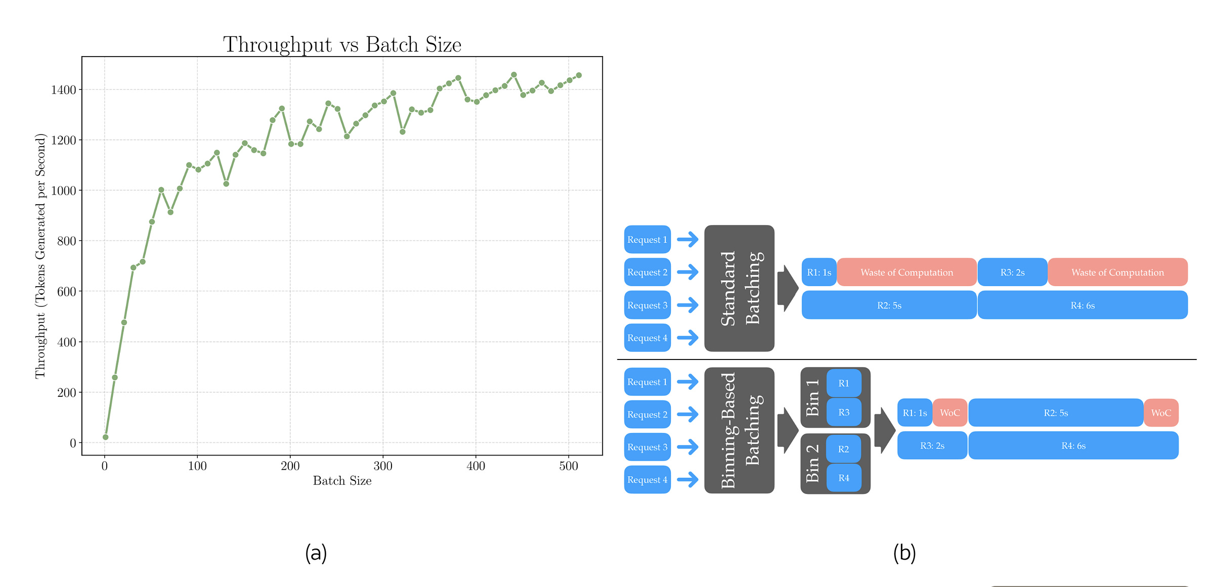
Length-aware bucketing: Sequences within a batch rarely have the same length. To align them, shorter sequences are padded with special padding tokens so they all match the length of the longest one. The catch: GPUs still compute on those padding tokens, burning cycles on useless work. Length-aware bucketing fixes this inefficiency by grouping requests of similar length into the same batch, so the amount of padding is minimized. The result is higher effective GPU utilization, faster inference, and reduced cost — without touching the model architecture or quality of outputs.

When it comes to batching, these are your triangle-armbar-guillotine-invert into heel hook combo— the reliable basics that will give you good enough returns in most cases. There are more advanced techniques here as well, but we will move on for now.

Batching is a very good field of applied research in AI and we will certainly be doing more deep dives into it.

1.2 Reducing Inference Overhead with Compiler & Graph Execution

Running an LLM under PyTorch (or TensorFlow) looks simple but under the hood, the framework issues thousands of separate GPU kernel calls for every forward pass. Each kernel does a small piece of work (normalize, multiply, apply bias, activate). Between kernels, results are written into global GPU memory (HBM), then read back.

(The term Kernel simply means a small GPU program that executes a single operation on a batch of data. Think of it as the atomic work unit that CUDA launches on the GPU.)

That memory is ~2–3 TB/s on an H100, which sounds vast — but registers (on-chip) are 10–50× faster. So every unnecessary write/read is wasted potential. Worse, each kernel launch goes through the CPU runtime. Launch overheads add up — tens of microseconds each — which, repeated thousands of times per token, becomes milliseconds of wall time.

If we can reduce the overhead in constantly checking for solutions, we’re in a very good place. Our next set of techniques focuses on this, raising the ceiling on throughput and reducing variance in latency.

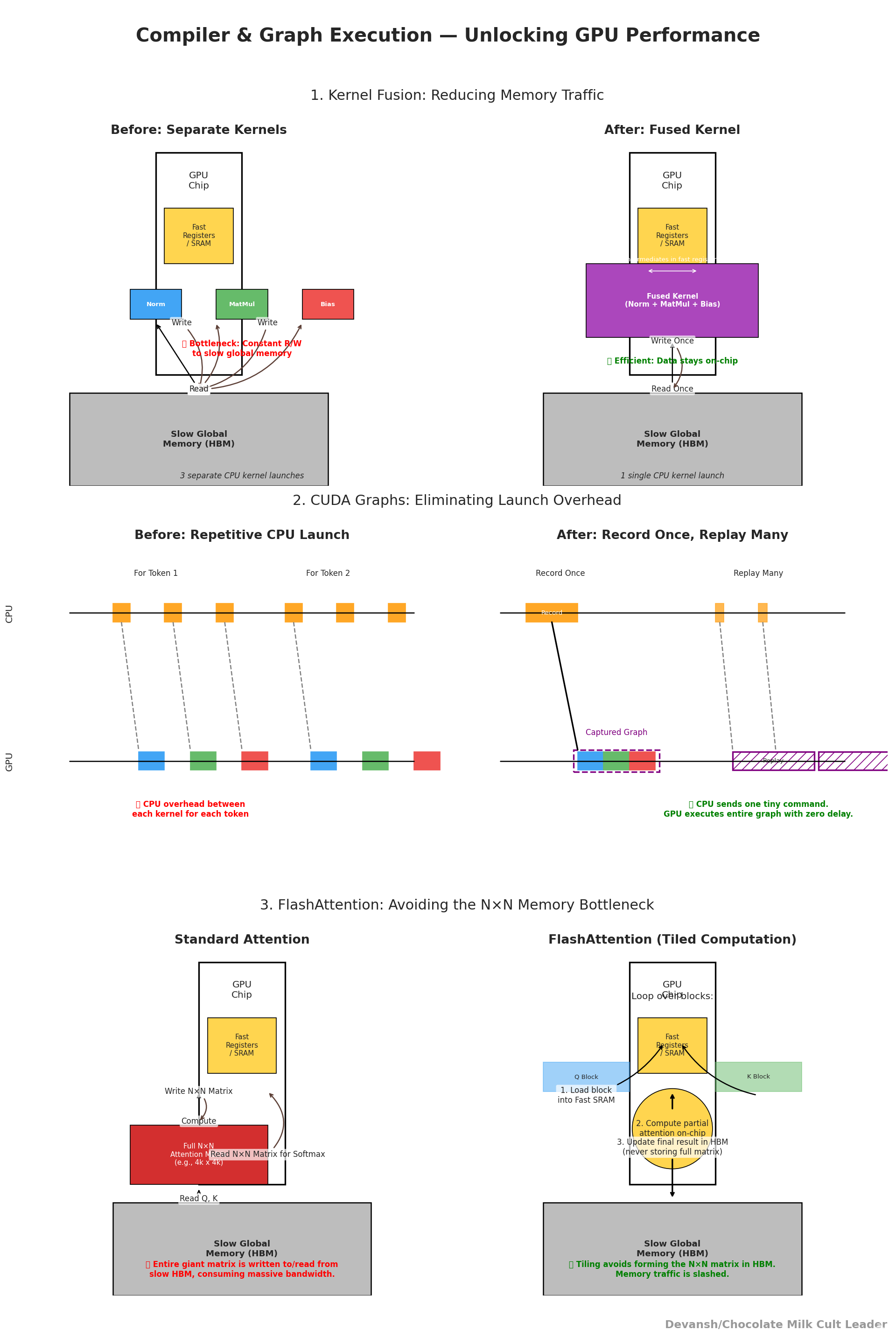
Kernel Fusion: Instead of launching three kernels — (1) LayerNorm, (2) QKV projection (a matrix multiply), (3) add bias — you fuse them into one.

How it works technically: The compiler rewrites the computational graph to combine operations with compatible shapes into a single GPU kernel. Intermediate results stay in registers or shared memory, never touching global HBM.
Impact: Cuts memory traffic, reduces kernel launches. This is especially valuable in deep transformers, where LayerNorm + linear projections occur hundreds of times.
Failure mode: Not all ops fuse cleanly. Irregular shapes (odd hidden sizes, dynamic padding) may block fusion. You end up with some fused, some unfused kernels.

I’ve been very interested in the memory wall and was curious about how some of the AI Hardware/Infra players could interact with Kernel Fusion. This is what I could tell from my early studies, but I’m happy to hear if you see this differently.

CUDA Graphs: Decoding involves the same sequence of kernels repeated once per token. Instead of launching those kernels through the CPU every time, you record them once, then replay the graph directly on the GPU.

How it works technically: The CUDA runtime provides an API for capturing a stream of GPU operations (with all dependencies resolved). Future calls reuse this pre-captured sequence, bypassing the CPU scheduler.
Impact: Eliminates launch overhead. On long sequences, this can save hundreds of microseconds per token, which compounds into milliseconds per generation.
Failure mode: CUDA graphs are tied to shapes. Change the batch size or sequence length, and the captured graph no longer applies. The trick is to capture graphs for the “hot” shapes (common sizes) and fall back gracefully otherwise.

Techniques like CUDA graphs are what allow Nvidia to bully the rest of the industry and charge their margins. We mentioned in previous live streams and market reports that Nvidia competitors were consolidating around building alternatives to CUDA.

“It’s really difficult to explain to non-programmers — or even programmers who don’t deal with massive compute problems — just how night-and-day the difference is between CUDA and its alternatives… But for stuff that is meant to run on “real” workloads to try to demonstrate cutting-edge performance on massive datasets, that’s in the CUDA ecosystem.
One can liken it to Adobe/Microsoft/AutoCAD software being used extensively in educational institutions, and that makes them also very sticky in industry (which in turn reinforces why schools use them). Of course, it’s even more painful to switch from CUDA in this case.”
-This article is a great read on why CUDA is a moat for Nvidia. Follow the brilliant
James Wang
for more like this

FlashAttention: Standard attention requires computing an N×N score matrix between queries and keys. For N=4k, that’s 16 million entries. The raw math isn’t the killer — it’s the fact that this matrix has to be stored in memory, read back, and used for softmax. That’s gigabytes of memory traffic per head, per layer, per token. FlashAttention addresses this.

How it works technically: FlashAttention tiles the computation. Instead of building the full matrix, it loads small blocks of queries and keys into on-chip SRAM, computes partial attention scores, applies softmax incrementally, and discards the intermediates. The final result (context vector) is correct to floating-point precision, but the memory bill is a fraction of the naïve algorithm.

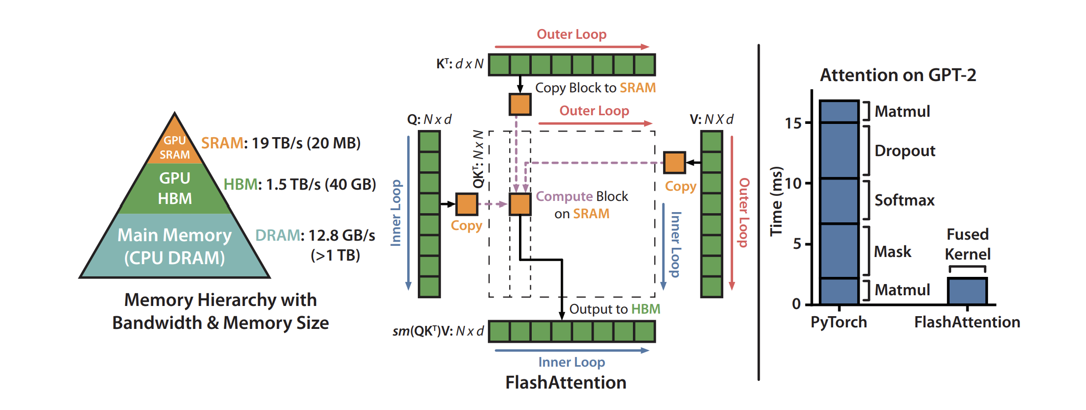
“Left: FlashAttention uses tiling to prevent materialization of the large 𝑁 × 𝑁 attention matrix (dotted box) on (relatively) slow GPU HBM. In the outer loop (red arrows), FlashAttention loops through blocks of the K and V matrices and loads them to fast on-chip SRAM. In each block, FlashAttention loops over blocks of Q matrix (blue arrows), loading them to SRAM, and writing the output of the attention computation back to HBM. Right: Speedup over the PyTorch implementation of attention on GPT-2. FlashAttention does not read and write the large 𝑁 × 𝑁 attention matrix to HBM, resulting in an 7.6× speedup on the attention computation.”

Impact: Cuts memory bandwidth by 3–5× and makes long-context attention feasible (tens of thousands of tokens).
Failure mode: Gains depend on sequence length. For very short sequences, FlashAttention may add overhead without saving much. That’s why good compilers dynamically switch kernels based on input size.

FA is a constantly being upgraded (although many of the upgrades are based on CUDA and not as transferable), so make sure you check the most relevant version to you.

“Flash Attention v4 at HotChips Conference which is up to 22% faster than the attention kernel implementation from NVIDIA’s cuDNN library. Tri Dao was able to achieve this 2 key algorithmic changes. Firstly, it uses a new online softmax algo to skip 90% of output rescaling. Secondly, in order to better overlap the softmax computation with the tensor core computation, it uses software emulation of exponential (MUFU.EX2) to boost throughput.”

Together, the 3 techniques play off each other wonderfully

Kernel fusion: fewer writes, more work per cycle.
CUDA graphs: no launch overhead; GPU stays in motion.
FlashAttention: no NxN memory blowup; bandwidth freed for other ops.

We can also tie them in very harmoniously with the next technique.

1.3 Doing less work for Inference with Quantization

Models store weights as 16-bit or 32-bit floats. But you don’t need that precision. As goated research like Microsoft’s Bitnet and MatMul Free LLMs show us, you can shave off a lot w/o hitting performance drop-offs.

BitNet b1.58 2B4T advances the Pareto frontier defined by leading open-weight LLMs under 3B parameters in terms of performance versus memory, demonstrating superior efficiency.

The technique.

Weight-only quantization (INT8/INT4): Store weights in 8-bit or 4-bit integers, scale them back up during computation. Sensitive parts (layernorm, softmax) stay in higher precision.

The team from Bitnets pushes this much further, but this can be harder to pull off for most teams.

FP8 math (on Hopper GPUs): Use 8-bit floats directly on tensor cores, halving memory footprint vs FP16 with negligible accuracy loss.

This has a relatively simple calculus: Smaller weights = less memory traffic = more tokens/sec. It also lets you fit bigger models on cheaper hardware. Just keep in mind that Quantization isn’t “free.” Calibrate poorly, and the model’s perplexity spikes; outputs degrade (hence why I only suggested weight only to lower precision). Done right, though, it’s invisible.

Once we apply this strong foundation, we’re ready to move on to the next level. But this leaves us with one final question. One that every AI team should ask when getting into a project. How do we know when enough is enough? What’s the exit criteria? This is key b/c technical people have a tendency to overengineer, optimizing a solution far past the point of good returns. Here are the rough guidelines we give to the teams in the chocolate milk cult.

Exit Criteria for this tier

You don’t leave Tier 1 until:

Prefill and decode are separated, both showing ≥75% GPU utilization.
Your decode loop is running as a CUDA Graph, not thousands of micro-launches.
Your quantized model runs with <1% regression on your evaluation set.

Meet these, and the GPU is finally working for you. And you’re ready to kick it at the next level.

Tier 2 — The Accelerants: Algorithmic & Memory Warfare

Tier 1 gave you a GPU that’s busy. Tier 2 is about lowering the cost of what that GPU is busy doing. This means we must now get past the Vidic-Fedinand gatekeeping of AI Inference: memory bandwidth (KV cache) and quadratic attention (sparsity).

Every decode step streams through gigabytes of cached state; every new token pair adds a fresh edge in the attention graph. All of this means that your memory can get crushed. These are the limits that turn trillion-parameter models into toys unless you fight them head-on.

So how do we fight? Glad you asked —

2.1 KV Cache Optimization — Taming the Memory Beast

Transformers store two vectors for each token at every layer: the key (K) and value (V). Together, these form the KV cache. Without it, every token would have to be recomputed from scratch. Using it taps the classic software engineering tradeoff — building solutions that save compute by using memory.

The formula is simple:

KV cache per layer = context length × hidden size × 2 × precision. The 2 here comes from the fact that we have to store both the K and V vectors.

Example:

Context length = 32,000 tokens
Hidden size = 4,096
Precision = FP16 (2 bytes per number)

That comes out to roughly 8 GB per layer. Multiply across 40 layers, and you’re staring at around 320 GB. And this isn’t just storage sitting around: every new token must read the entire cache for its attention step. That means gigabytes streamed per decode step. Here, you can no longer worry about FLOPs, since your memory bandwidth will Yamcha your systems much sooner.

When it comes to Techniques to shrink or tame the cache, I like to group them by the level they operate at. Structure-level tricks remove duplication, representation-level tricks shrink each entry, and policy-level tricks bound growth outright. Used together, they turn a 320 GB monster into something tractable.

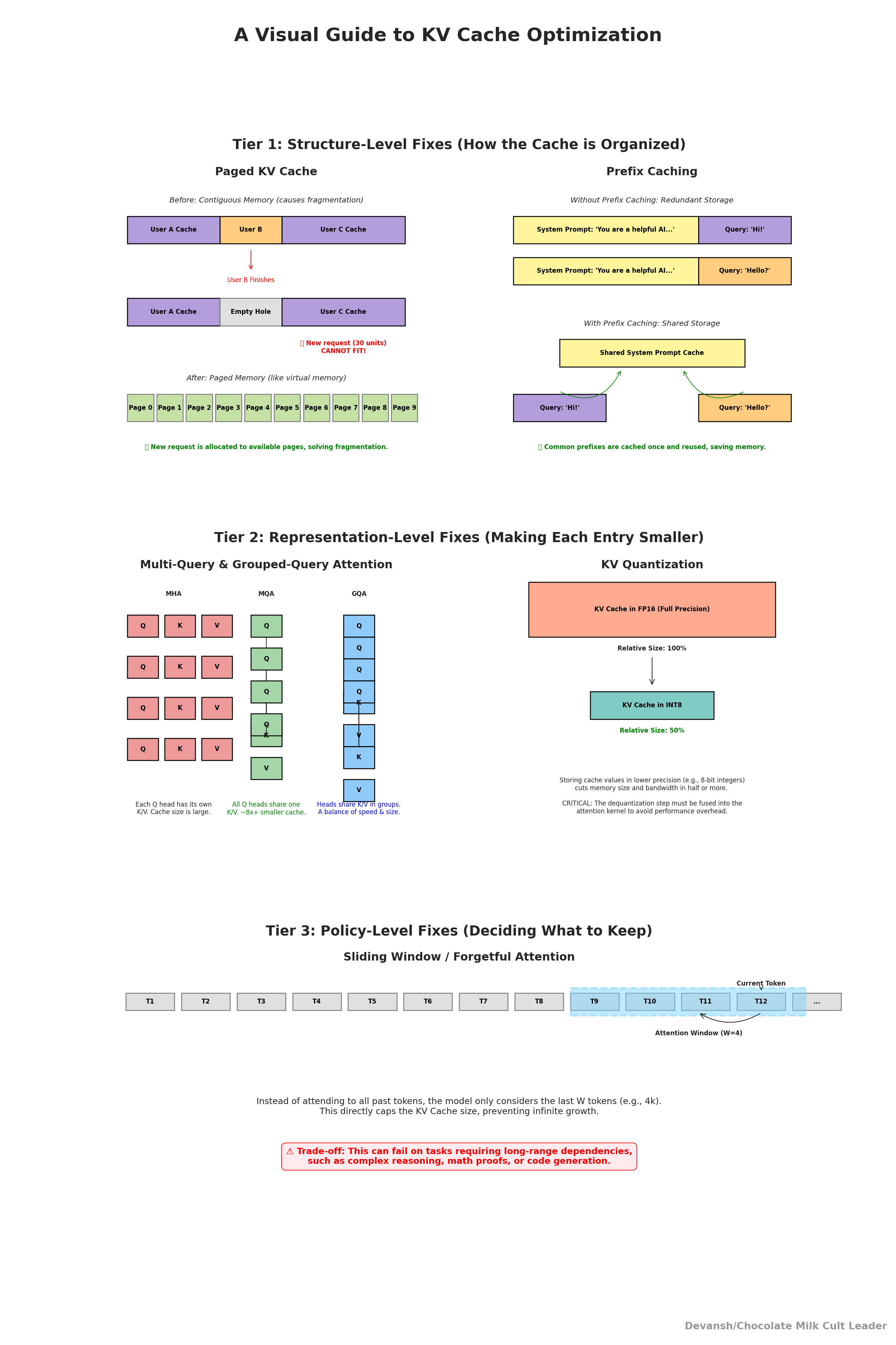
Structure-level fixes (how the cache is organized):

Paged KV: Split the cache into fixed-size pages, like virtual memory. This makes it easier to reuse common prefixes and prevents memory fragmentation. Instead of duplicating a giant block, you reuse pages.
Prefix caching: In chat systems, the opening prompt or system instructions repeat constantly. Cache them once and point subsequent requests at the same data. The challenge is normalization: tiny differences (like timestamps, whitespace, or IDs) can break cache hits unless you clean them first.

Representation-level fixes (make each entry smaller):

Multi-Query or Grouped-Query Attention (MQA/GQA): Normally, every head has its own K and V. With 32 or 64 heads, that means 32 or 64 copies of the same information. MQA shares one K/V across all heads, and GQA shares across groups of heads. This can reduce cache size by 8× or more.
KV quantization: Store K/V in int8 or int4 instead of FP16. This cuts storage and bandwidth by half or more. But to work, the dequantization must be fused into the attention kernel — otherwise you waste the savings on overhead.

Policy-level fixes (decide what to keep at all):

Sliding window or forgetful attention: Instead of attending to every token ever generated, limit attention to the last W tokens. For many use cases, W between 4k and 16k is plenty. This caps memory growth directly. But beware: tasks like code generation, legal reasoning, or math proofs can collapse if you drop long-range dependencies. This one of the difficulties of context management, especially when you consider that some tasks require you to hold entire documents in memory (at Iqidis our users often upload a document and try to turn it into a template for other drafts; this requires keeping the entire doc and later the template in memory).

Without KV optimization, context scaling stalls around 8k–16k tokens. With it, 100k+ contexts become realistic and commercially viable.

2.2 Sparse Architectures — Activating Only What’s Necessary

Vanilla Transformers are dense:

Every parameter in the model fires on every token. So FLOPs scale linearly with model size.
Every token attends to every other token. So FLOPs scale quadratically with context length.

This is fine at small scales, but lethal at the frontier. A trillion-parameter dense model or a 100k-context dense transformer is an academic toy — impressive, but unusable in practice.

Sparsity is how you break this link. It lets you add capacity or length without paying dense costs. Here, we can explore two orthogonal approaches —

2.2.1 Mixture-of-Experts (MoE) — parameter sparsity.

MoEs are networks composed of “expert” sub-networks and a “gating” network that dynamically routes inputs to the appropriate experts. This allows for conditional computation, making large networks more efficient-

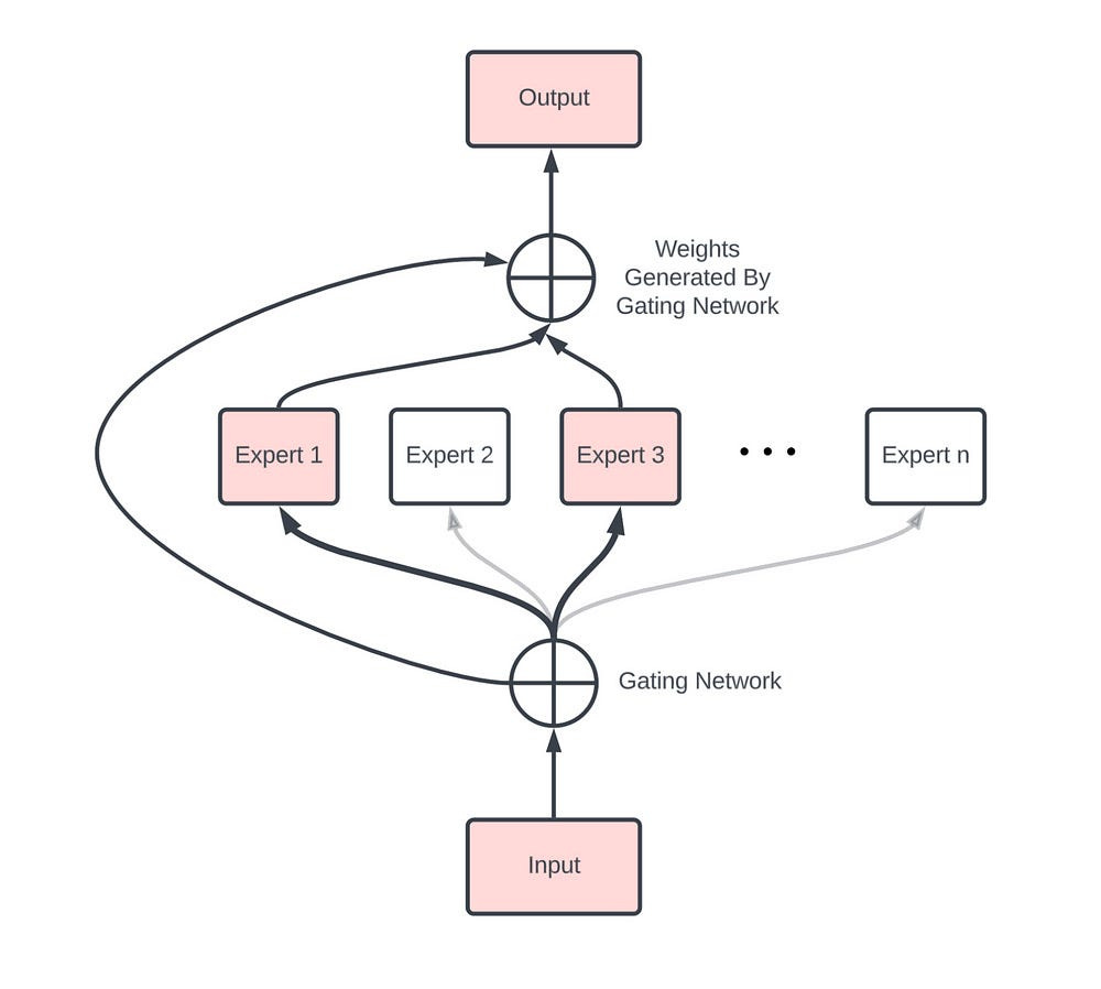
This allows trillion-scale capacity with a fraction of the compute per token, if their needs can be met. MoE depends on fast all-to-all interconnects. Routing tokens to experts requires moving data across devices quickly. Without a high-bandwidth interconnect, MoE stalls.

Unfortunately, MoEs come with a whole host of failure conditions —

Load imbalance (some experts overused, others idle)
Router instability,
Communication bottlenecks b/w modules.
To reiterate, MoEs aren’t the best for stability (an idea we explored in our critiques of Gemini here), making them very volatile if not designed correctly.
Look no further than Meta’s mess with Llama 4. Despite their money and talent (and major open LLMs that had done MoE), Meta still struggled to run the MoE well.

Breathtaking when functional (but often isn’t), unstable, and needs a lot of communication. Remind you of anyone?

2.2.2 Sparse Attention — activation sparsity.

Standard attention complexity is quadratic: number of tokens squared. At 32k tokens, that’s over a billion pairwise interactions per head. Sparse attention cuts this by restricting patterns:

Sliding windows: each token looks only at the most recent tokens.
Local + global: most tokens look nearby, a few tokens are designated as global anchors. This seems like a winning play across AI (LSTMs do this for weather; I’ve heard Vision Transformers do something similar when they get doped with ConvNet Features as well — the former being more global while the latter adding the locality).
Block sparsity: the sequence is chunked, with only limited cross-block links.
This reduces cost to linear or near-linear, making very long contexts feasible.

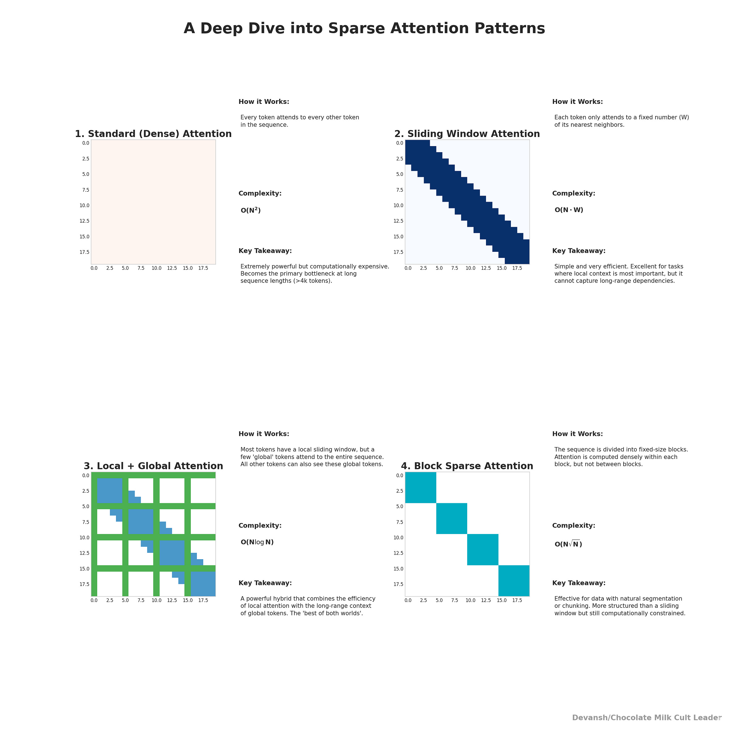
The types of Sparse Attention visualized.

This only works if kernels are efficient. If your implementation falls back to dense operations, you gain nothing. Global-dependency tasks — retrieval, theorem proving, code generation — can break if sparsity is too aggressive.

Taken together, MoE and sparse attention attack different axes:

MoE sparsifies parameters (breadth of the model).
Sparse attention sparsifies activations (length of the sequence).

They can be combined. Together, they are the only way to serve trillion-parameter models with 100k contexts at anything like usable cost. Sparsity is one of the earliest signals we flagged for LLM development, all the way back in May 2022 (many months before ChatGPT), in our breakdown of Google’s pathways architecture. I’ve monitored it since then, and interestingly, there hasn’t been a lot of core innovation in this area (we’ve optimized processes; not rethought assumptions). This seems like an area with a lot of untapped alpha, and would encourage any builders/researchers to start playing with Sparsity.

This is the snippet from the Pathways deepdive. The same deep dive also looks at multi-modality. We were catching next-gen trends before LLMs were a term.

2.3 How to Reduce LLM Inference Costs with Speculative Decoding

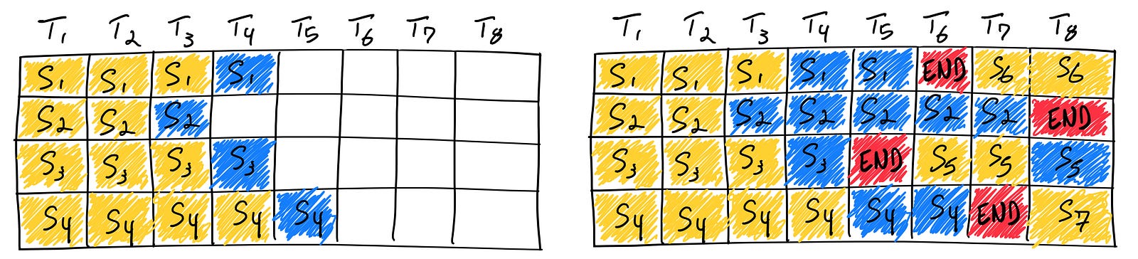
LLMs, by their nature, generate text one token at a time. Predicting the next token requires knowing all preceding tokens. This sequential dependency creates inherent latency. On top of this, each token prediction necessitates a full forward pass of the model. This is not only slow, but also expensive since your costs scale linearly with the output sequence length. Spec Decoding is a technique that can help you speed up your outputs dramatically-

Notice how quickly Spec Decoding hits breakeven.

How Speculative Decoding Works

Speculative Decoding works in the following way-

Draft Model (Small and Fast and Cheap): A smaller, faster “draft” model is employed. Crucially, this model is also significantly cheaper to run than the main (“target”) LLM.
Speculative Generation (Draft Model): The draft model takes the current sequence and, in parallel, proposes multiple future tokens (say, k tokens).
Verification (Target Model/Main LLM): The target LLM then performs a single forward pass, but over the original context plus the k speculated tokens.
Acceptance/Rejection (Statistically Sound Validation): The target model’s output probabilities are compared to the draft model’s. Accepted tokens are kept; rejected tokens are replaced with the target model’s predictions, and subsequent speculations based on rejected tokens are discarded. The key is the statistically sound acceptance criterion that maintains the output distribution’s integrity.
Iteration: The process repeats, starting from the last accepted token.

The process is shown below-

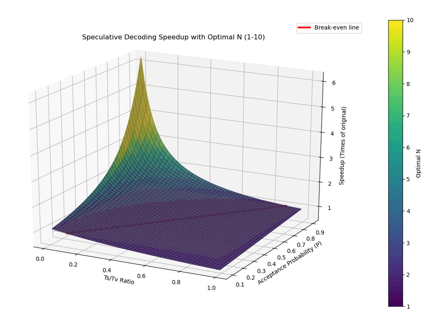
How Speculative Decoding Cuts Costs

Spec Decoding relies on the assumption that, on average, a good portion of the draft model’s speculations are correct. This means that a good portion of the inference is done by a much smaller and cheaper model. Instead of paying for k target model passes, we pay for 1 target model pass and k (much cheaper) draft model passes. Since the draft model is significantly smaller and faster, the overall cost per generated token is substantially reduced.

“In our original paper, we demonstrated the efficacy of this approach through application to translation and summarization tasks, where we saw ~2x–3x improvements. Since then, we have applied speculative decoding in a number of Google products, where we see remarkable speed-ups in inference, while maintaining the same quality of responses. We have also seen speculative decoding adopted throughout the industry, and have witnessed many insightful and effective applications and ideas using the speculative decoding paradigm.”
-Looking back at speculative decoding.

The benefits of Spec Decoding have led to a lot of research in improving the solution further. The primary limitation of that approach — the need to train and host a separate draft model — has been addressed by several innovative draft-model-free variants that are now state-of-the-art:

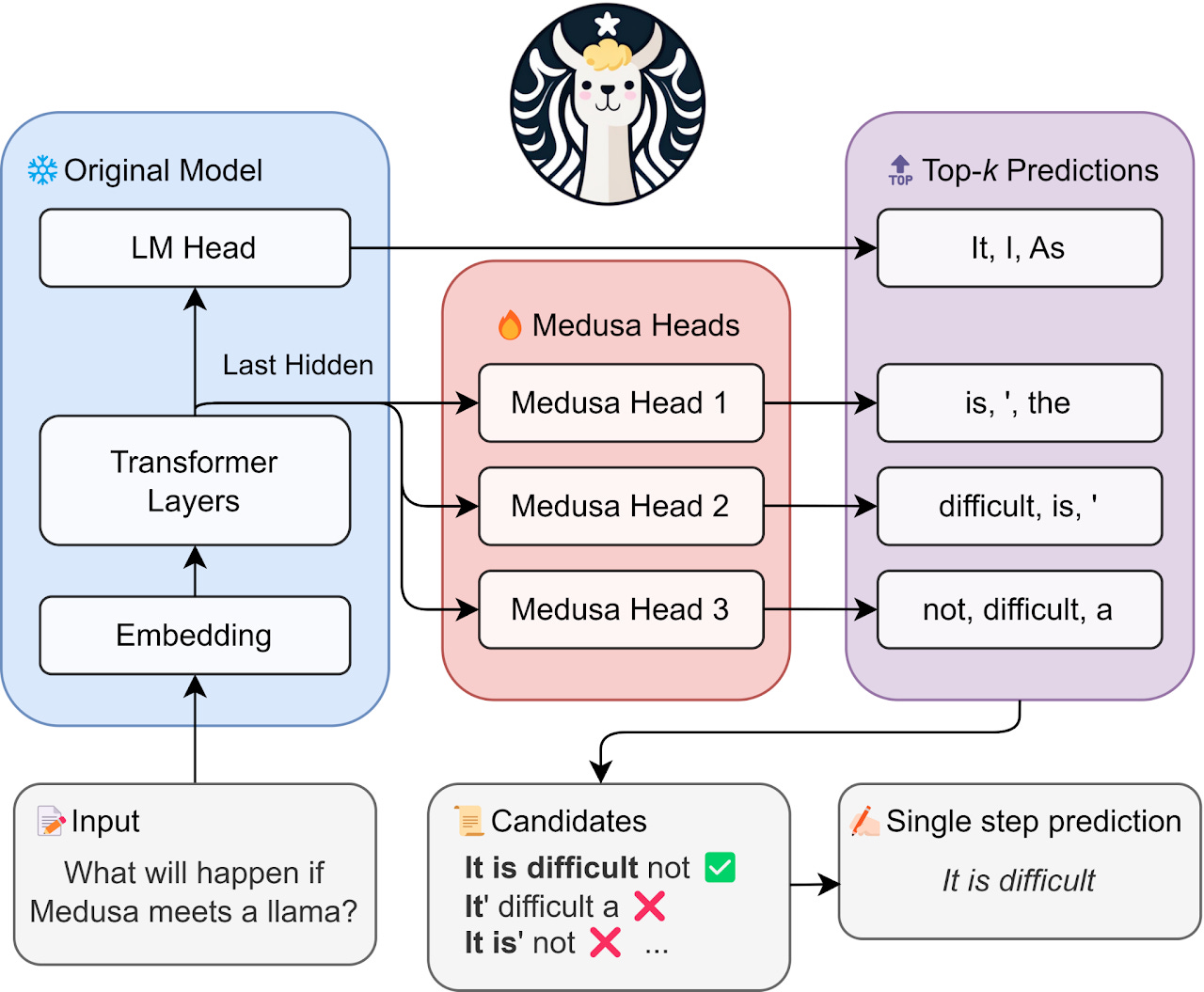
Medusa: This approach eliminates the separate draft model by augmenting the target model with multiple, lightweight “decoding heads”. Each head is a small neural network attached to the final layer, trained to predict tokens at future positions (e.g.,n+1, n+2, etc.). During inference, these heads generate multiple candidate continuations in parallel, which are then organized into a tree and verified by the target model in a single forward pass using a specialized “tree attention” mechanism. This keeps the entire process within a single model, simplifying deployment.

**“Overview of Medusa.** Medusa introduces multiple heads on top of the last hidden states of the LLM, enabling the prediction of several subsequent tokens in parallel. When augmenting a model with Medusa heads, the original model is frozen during training, and only the Medusa heads undergo fine-tuning. This approach makes it feasible to fine-tune large models on a single GPU. During inference, each head generates multiple top predictions for its designated position. These predictions are assembled into candidates and processed in parallel using a *tree-based attention* mechanism. The final step involves utilizing a *typical acceptance* scheme to select *reasonable* continuations, and the longest accepted candidate prefix will be used for the next decoding phase. The efficiency of the decoding process is enhanced by accepting more tokens simultaneously, thus reducing the number of required decoding steps.”

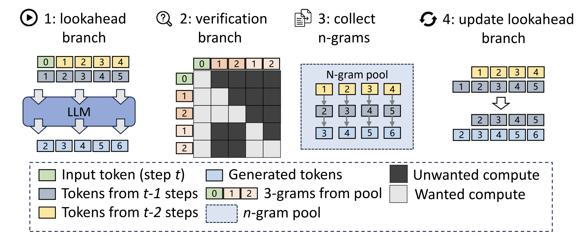
Lookahead Decoding: This technique also operates without an auxiliary model. It is based on the insight that an LLM can generate multiple disjoint n-grams in parallel. Lookahead decoding uses a mathematical technique related to Jacobi iteration to generate candidate n-grams for future positions and then verifies them against the model’s standard autoregressive output, all within a single computational step. It achieves speedups of 1.5x to 2.3x without the complexity of a two-model system.

“Workflow of LOOKAHEAD DECODING with W = 5, N = 3, and G = 2. For each decoding step, we do the following. (1) Generate one token at each position in the lookahead branch; (2) Verify and accept 3-grams (searched from the 3-gram pool) with the verification branch; (3) Collect and cache newly generated 3-grams in the pool from lookahead branch trajectories. (4) Update the lookahead branch to maintain a fixed window size.”

If you’re going to implement Spec Decoding, here are useful tips that would help you-

Cost-Aware Thresholds: When adapting the acceptance threshold dynamically, factor in the cost implications. In situations where cost is paramount, you might be willing to accept a slightly lower acceptance rate (and thus slightly reduced quality) to achieve greater cost savings.
Chunking and Cost: Phrase-level or chunk-level speculation speeds up generation and amortizes the cost of the target model’s forward pass over a larger number of tokens, further reducing the cost per token.

From what I hear, pretty much every major AI Lab is either already adopting or experimenting with Spec Decoding. No reason for you to be far behind. I believe in you. Especially w/ many breakthroughs around the new way of cheap models that are operating at a new Pareto frontier; redefining the performance per dollar we can expect in AI (look no further than Google’s investment into Gemini Flash for proof why it’s so important)

Exit Criteria for Tier 2

You don’t graduate until:

KV cache bandwidth is under control, and prefix reuse shows up in logs.
Speculative decoding shows ≥2× end-to-end speedup, not just draft-model dreams.
Sparse methods give real throughput gains without wrecking performance on long-range tasks.
Context windows beyond 32k run stably, without thrashing memory or collapsing throughput.

Tier 3 — The Final Frontier of Inference Scaling

Tier 3 is about the leftovers — the marginal costs that still drain your system at scale. These are not obvious bottlenecks like FLOPs or HBM bandwidth. They’re death-by-a-thousand-cuts: invalid outputs bloating your cache, bloated models you can’t afford to serve, tail latency hiding in your topology.

3.1 Constrained Decoding — Forcing Correctness

Every invalid token costs real money. Generating an invalid JSON bracket still required:

A full softmax over the vocabulary (tens of thousands of logits).
An append to the KV cache (expanding memory and bandwidth).
A wasted pass through your decoding loop.

Constrained decoding masks impossible tokens at generation time:

JSON schema enforcement (only allow tokens that keep JSON valid).
Regex masks for structured strings (emails, phone numbers).
Trie-based vocab pruning (whitelist of valid outputs).

This ups both Correctness — invalid-output rate drops toward zero — and Efficiency — fewer retries, shorter traces. In enterprise chat workloads, constrained decoding can cut generation length by 15–20%.

As long as you can handle the additional engineering (and subsequent debt), this is a very helpful tool, especially for selling in low-error scenarios where little details often matter disproportionately.

3.2 Distillation & Pruning for Lower Inference Costs

Even after Tier 2 tricks, a bloated model burns money. A 13B dense model consumes double the VRAM of a 7B. That halves your batch size and doubles your $/token. At edge or mobile, it’s impossible to deploy.

Distillation.
Train a smaller “student” to mimic a large “teacher.”

Logit distillation: student matches the teacher’s probability distributions. This is the most effective version of distillation, and ≥80% of your distillation budget should go here.
Response distillation: student mimics outputs directly.
Alignment distillation: students inherit guardrails from bigger aligned models.

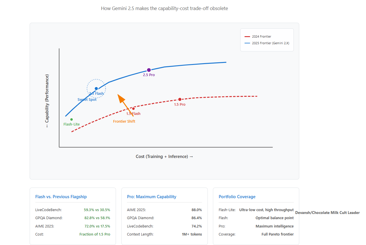
My favorite model in the market (2.5 Flash) is a great example of the effectiveness of distillation. It distills the best AI in the market (2.5 Pro) to get an insane performance per dollar.

Pruning.
Remove weights that don’t matter.

Magnitude pruning: drop smallest weights.
Structured pruning: cut entire channels or neurons.
N:M sparsity: enforce patterns like “2 of every 4 weights nonzero” so hardware kernels can exploit it.

On GPUs that support 2:4 sparsity, pruning can yield 1.5–2× throughput boosts without retraining from scratch.

The risks here are clear, so we won’t spend too much time on them. You need to focus on monitoring drift and ensuring that your pruning is set up properly.

3.3 Algorithmic Shortcuts through Verifiers

Inference costs explode because every token walks through the full depth of the model. Early-exit schemes and speculative decoding try to dodge this by doing less work — but both raise the same question: who decides when “less” is enough?

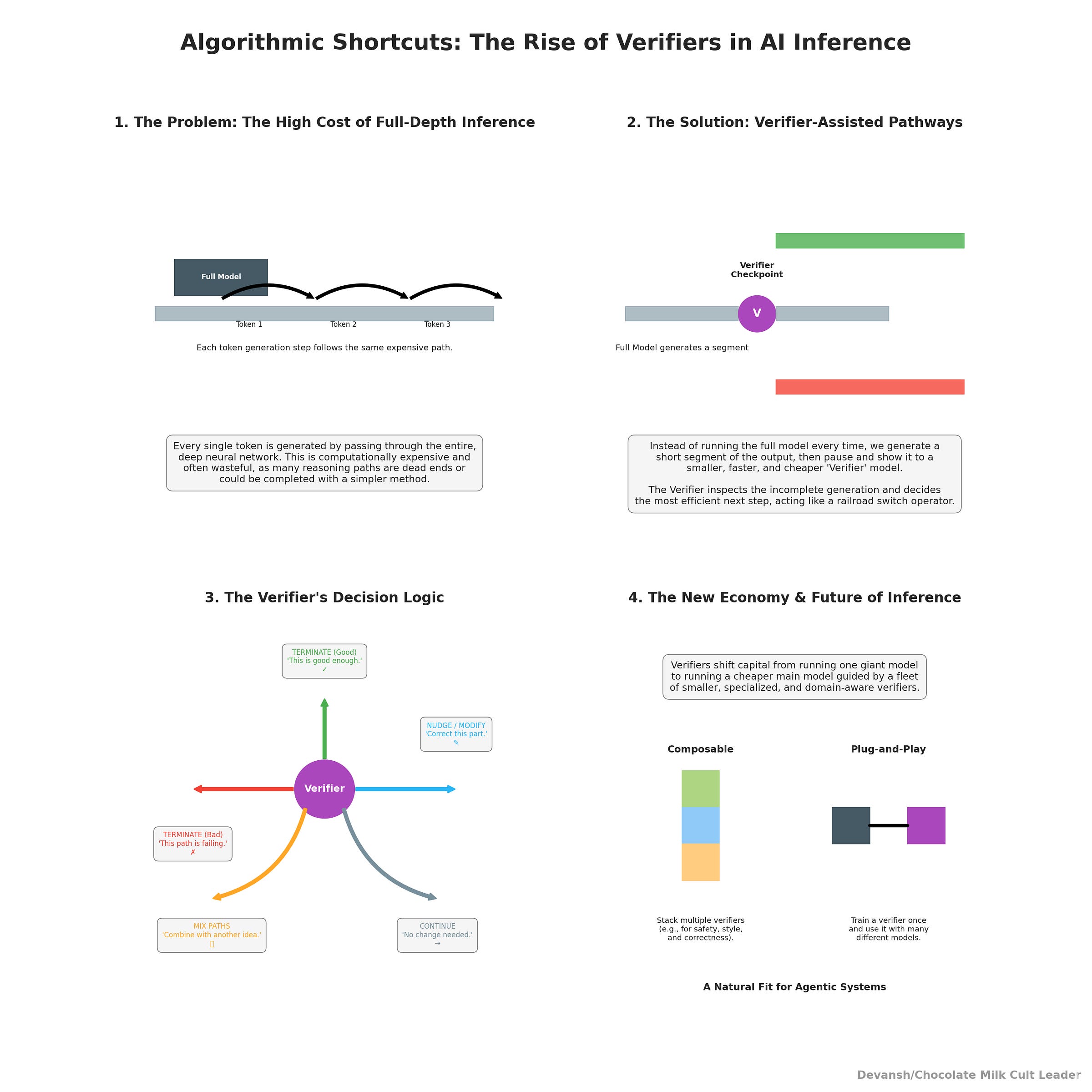
That’s where verifiers come in. Verifiers are reward and scoring models that look at incomplete generations and decide whether this is worth doing. Based on the looks of the output, your verifier might —

Terminate a path because it’s good enough and return answers.
Terminate a reasoning path b/c it’s not good at all, and let the model explore alternatives.
Nudge the model to modify the path.
Decide to modify the path by mixing with other paths.
Continue down the path with no changes.

This obviously requires domain-aware verifiers, which means that you’re shifting capital from pure decoding to both building and running verifiers. However, imo verifiers will be one of the biggest shifts in the economy, especially since they can be composed (combine multiple verifiers), plug and played (train a verifier and use it somewhere w/o training an entire model), and are a natural fit for agentic systems (and for regulated spaces). Iqidis is already using them to assess and guide legal case strategy, and the results have been amazing. We were even mentioned in MEALEY’S International Arbitration Report specifically for this capability-

“The leap is even clearer with expert evidence. Industry platforms such as Iqidis can do far more than redline comparisons. They test underlying assumptions, spotlight methodological gaps, and chart precisely where two experts diverge. In technical disputes involving — for example — construction, energy, or financial products, that context turns a scattershot cross-examination into a surgical one.”

3.4 Topology for Inference Scaling

Even the best-optimized model lives in a system: GPUs, CPUs, memory, networks. Where you place things dictates latency and throughput. Bad placement silently wrecks performance.

Here is what to look for —

Model–data co-location. Put LLM servers and vector databases in the same rack. Cross-rack hops add milliseconds to every request, ballooning tail latency.
NUMA awareness. On multi-socket hosts, memory belongs to CPUs. If your GPU worker is pinned to the wrong socket, every transfer drags across NUMA lanes. That’s wasted microseconds per token.
Replica vs. Shard. Replicas (each GPU runs a full copy) keep latency low but cost VRAM. Shards (model split across GPUs) save VRAM but every inference step is a cross-GPU conversation. Latency balloons.
Response caching. Cache completions close to where prompts land. In enterprise chat, 30–50% of requests can hit cache if prompts are normalized, eliminating millions of tokens/day.

Topology is invisible until it fails. Then it’s everything. A poorly placed system doubles your P99 latency, even if your model is flawless. Get placement right, and your infra bill drops without touching a single weight.

3.5 Policy Tuning

Tuning temperature, top-k, or penalties isn’t only about style. It changes sequence length. A poorly tuned sampler can add 10–20% more tokens per output. Multiply that by billions of tokens/month, and you’re burning GPUs for nothing.

Exit Criteria for Tier 3

You don’t move on until:

Invalid-output rate in structured tasks is below 0.1%. If not, your decoding isn’t constrained.
Distilled/pruned models run at least 30–50% cheaper per token than their teachers. If not, your “surgery” is cosmetic.
Response cache hit rates are ≥25% in production. If not, your normalization is broken.
Tail latency (P99) is stable after topology tweaks. If not, your placement is wrong.
Average tokens per output fall after decoding policy tuning. If not, you’re wasting spend.

Conclusion — Scaling for Whom?

Scaling is rarely framed honestly. At its core, it rests on a quiet assumption: the future is just “more of the same.” Bigger models, longer contexts, higher throughput — an endless treadmill. But who does that vision serve?

Hyperscalers and infra giants profit from it. Every new token, every longer context, every optimization that keeps us inside their rails compounds their lock-in. For them, the treadmill is the business model.

For the rest of us — builders, users, communities — the picture is murkier. Some scaling breakthroughs clearly help: cheaper inference, better latency, wider access. But much of it risks entrenching the status quo, not expanding our agency. A quick read through history shows us that two things can happen at once —

The power/autonomy for an ordinary person increasing, letting them do more.
The power of an elite increasing disproportionately, increasing inequality.

An ordinary person can now do so much more than a medieval peasant, but at the same time, they are much more locked into society and can’t truly escape (even living in a jungle off the grid exposes one to global warming, poisoned water, destroyed ecosystems, etc).

That leaves the harder question: how can we ensure that the benefits of scaling are not chains keeping us tied to Plato’s cave? And how do we thrive inside the current system —building on the advantages of scaling — while also imagining an alternative future that brings power back to us instead of concentrating it further away?

If you will indulge me a bit more, we could even extend this line to ask a question — is it possible to be just while participating in an unjust system? What would that mean? Would love to hear your thoughts on this.

Thank you for being here, and I hope you have a wonderful day,

Chichora #1,

Dev <3

If you liked this article and wish to share it, please refer to the following guidelines.

That is it for this piece. I appreciate your time. As always, if you’re interested in working with me or checking out my other work, my links will be at the end of this email/post. And if you found value in this write-up, I would appreciate you sharing it with more people. It is word-of-mouth referrals like yours that help me grow. The best way to share testimonials is to share articles and tag me in your post so I can see/share it.