
The Real Cost of Running AI
From FLOPs to GPUs to KV Cache — What Every Token Actually Costs

It takes time to create work that’s clear, independent, and genuinely useful. If you’ve found value in this newsletter, consider becoming a paid subscriber. It helps me dive deeper into research, reach more people, stay free from ads/hidden agendas, and supports my crippling chocolate milk addiction. We run on a “pay what you can” model—so if you believe in the mission, there’s likely a plan that fits (over here).
Every subscription helps me stay independent, avoid clickbait, and focus on depth over noise, and I deeply appreciate everyone who chooses to support our cult.
PS – Supporting this work doesn’t have to come out of your pocket. If you read this as part of your professional development, you can use this email template to request reimbursement for your subscription.
Every month, the Chocolate Milk Cult reaches over a million Builders, Investors, Policy Makers, Leaders, and more. If you’d like to meet other members of our community, please fill out this contact form here (I will never sell your data nor will I make intros w/o your explicit permission)- https://forms.gle/Pi1pGLuS1FmzXoLr6
At the core of many AI discussions is the question: will AI ever pay for itself? Investors, CFOs, and builders all ultimately need to know what the cost of training and running AI is.
So far, the discussions around this have been very high-level, relying on simplifications. Cost models jump straight to macro numbers: “$X per token,” “$Y per data center,” “Z% margin,” while researchers are too scared to add a dollar value to the time complexity calculations they do. Unfortunately, that’s not good enough when it comes to making informed decisions in what AI is worth investing in, how much should be invested, and what challenges are we likely to encounter.
If we want to understand the economics of modern AI — why inference costs what it costs, why latency behaves the way it does, why certain architectures dominate the edge while others struggle — we have to trace the chain all the way down. We need deeper discussions on much more specific questions like —
How much does one attention head cost?
What does adding four layers do to memory traffic?
How does a different activation function change FLOPs?
What is the marginal bandwidth cost of extending context length?
How does KV cache growth alter revenue per GPU?
This piece walks through the entire value chain carefully, from first principles. We’re going to look deep into the mathematical details of every major AI operation, from self-attention to the costs of KV cache explosions, all to help you answer a simple question: What exactly are we paying for when we pay for intelligence?
We will cover:
How self-attention is constructed from basic linear algebra
The exact FLOPs per transformer layer
Why prefill and decode live in completely different hardware regimes
When performance becomes compute-bound versus memory-bound
How KV cache growth caps concurrency
How all of the above collapse into cost per token
The crossover math for edge vs. cloud — the MAU threshold where on-device deployment wins.
and more
Beyond understanding the basics of matrix multiplication, you won’t need to know anything else. We will dig into all of it from scratch so you can understand where every dollar you invest in AI actually goes. By the end, you will have the foundation for understanding what is coming next (which will be the basis of future explorations).
Let’s do this.

Executive Highlights (tl;dr of the article)
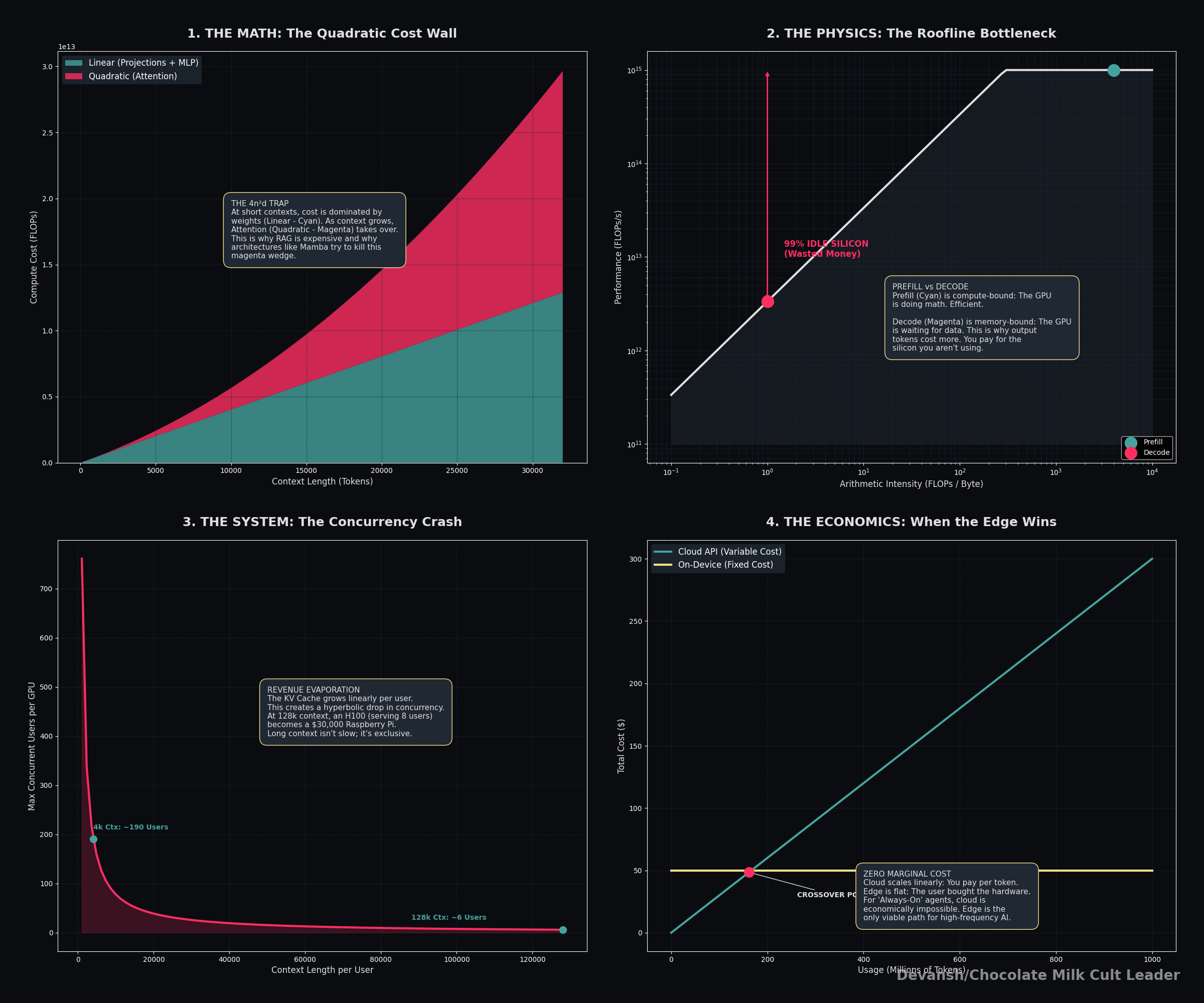
The transformer’s cost isn’t mysterious — it’s one formula: 24nd² + 4n²d per layer. The first term is linear in context and mostly unavoidable. The second term is quadratic in context and is the entire reason long-context inference is expensive, why RAG isn’t dead, and why every alternative architecture project is really just trying to kill that 4n²d term.
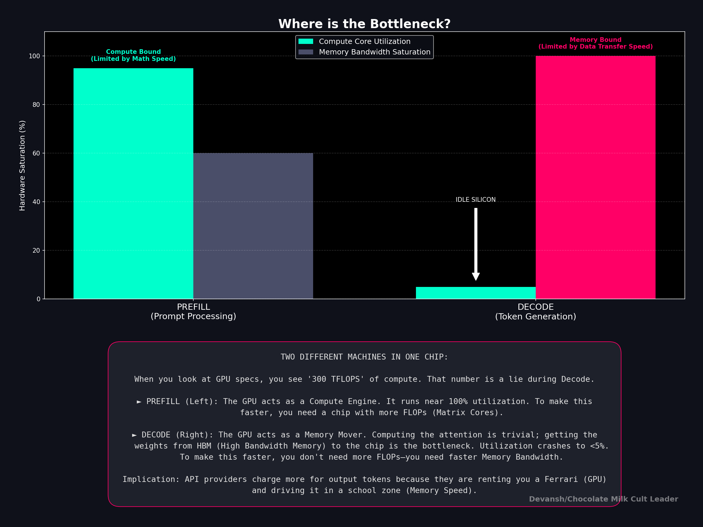
Prefill and decode are not the same workload running on the same hardware. Prefill is compute-bound (arithmetic intensity ~4096 FLOPs/byte on a 4K prompt) — the GPU is doing what it was designed for. Decode is memory-bound (arithmetic intensity ~1 FLOP/byte) — the most expensive chip in the world is running at 1% utilization while you pay full price. Output tokens cost more than input tokens because of physics, not margin.
The roofline model proves why decode can’t be fixed by buying better hardware. Every chip has two independent limits: peak compute and memory bandwidth. Prefill’s arithmetic intensity (~4096 FLOPs/byte at 4K context) sits deep in compute-bound territory — the H100 is doing what it was designed for. Decode’s arithmetic intensity collapses to 1–4 FLOPs/byte regardless of model size, context length, or architecture. The H100’s threshold is 295. You’re running at 1% of theoretical peak during the phase users are actually waiting on. Doubling the chip’s FLOPs changes nothing — decode is bottlenecked by memory bandwidth, not math, and memory bandwidth scales at roughly half the rate compute does. This isn’t a current-hardware quirk; it’s a structural mismatch that gets worse with every GPU generation. The entire inference chip startup ecosystem (Groq, Cerebras, Etched) is a direct bet against this single number.
The KV cache is the only cost component that scales with usage and varies per user — which makes it the single most important variable in inference economics. At 32K context, one concurrent user’s cache approaches the size of the model weights themselves. Double the context, halve your concurrent users. That relationship is linear and there is no architectural trick that changes it without eliminating attention layers entirely.
The raw compute floor for a well-optimized 14B-class deployment is ~$0.004/M tokens at full utilization. APIs charge $0.30–$1.25/M. That gap isn’t margin — it’s the cost of actually running a production service. But it also tells you the utilization lever is worth more than most architectural optimizations: same hardware, 10% utilization vs 30% utilization is a 3x cost swing before you change a single weight.
Edge isn’t cheaper cloud. At 100M MAU the per-token costs are comparable. At 500 requests/user/month the on-device cost is 11x cheaper — and more importantly, it’s flat regardless of usage growth. Always-on AI (ambient assistants, real-time translation, continuous summarization) is economically impossible on cloud metering. The architectural constraint isn’t capability, it’s extracting sufficient quality from sub-3B models at INT4.
Every serious architectural innovation of the last two years — GQA, hybrid attention/SSM, sliding window, MoE — is attacking the same two numbers: bytes of KV cache per token, and bytes of weights loaded per decode step. If a new architecture doesn’t move one of those, the economics don’t change regardless of what the paper claims.
I put a lot of work into writing this newsletter. To do so, I rely on you for support. If a few more people choose to become paid subscribers, the Chocolate Milk Cult can continue to provide high-quality and accessible education and opportunities to anyone who needs it. If you think this mission is worth contributing to, please consider a premium subscription. You can do so for less than the cost of a Netflix Subscription (pay what you want here).
I provide various consulting and advisory services. If you‘d like to explore how we can work together, reach out to me through any of my socials over here or reply to this email.
1. How Self-Attention Is Built (And Billed)
To understand what you’re paying for in AI, you have to isolate the most expensive component in the machine. In a transformer, that component is called (multi-headed) self-attention. Every aspect of computation, memory traffic, and cost somehow touches MHA.
At its core, MHA is a brilliantly elegant solution to a very hard problem: how does a machine understand that the word “bank” means something completely different depending on whether “river” or “account” appears nearby?
The simplest approaches fail immediately. You could average nearby tokens — but then “the dog bit the man” and “the man bit the dog” produce identical representations. You could concatenate fixed windows — but then a pronoun can never resolve its referent if the noun is outside the window. What you need is a mechanism where each token can dynamically look at the entire sequence and selectively extract the information it needs.
It should come as no surprise to you that we’re going to be spending a lot of effort building our intuitions for why MHA is the way it is.
1.1 The Raw Material: Language as a Table
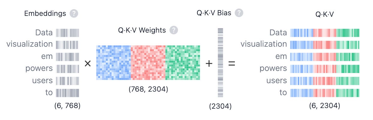
To do any AI, we need to represent language in a way a computer can process. We turn our input — a sentence, an article, a piece of code — into a simple table of numbers, a matrix we’ll call X.
This table has n rows, one for each token (or word). It has d columns, representing the vector of features that define that token. For a model like Llama 3.2–1B, d=2048.
(the formulation as tables means we may eventually see the GOAT, Excel enter the LLM ecosystem as a means of manipulation of latents, which might just be the missing piece for all AGI).
So, X is an n × d matrix. That number, 2048, gets squared in almost every cost formula we will derive, so pay it very close attention. The fundamental challenge is figuring out how each row in this table should communicate with every other row to build up a sense of context.
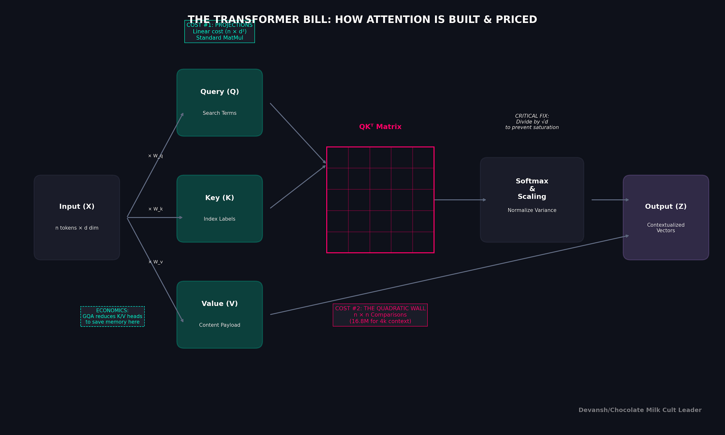
1.2 Q, K, V: The Cost of a Search Engine
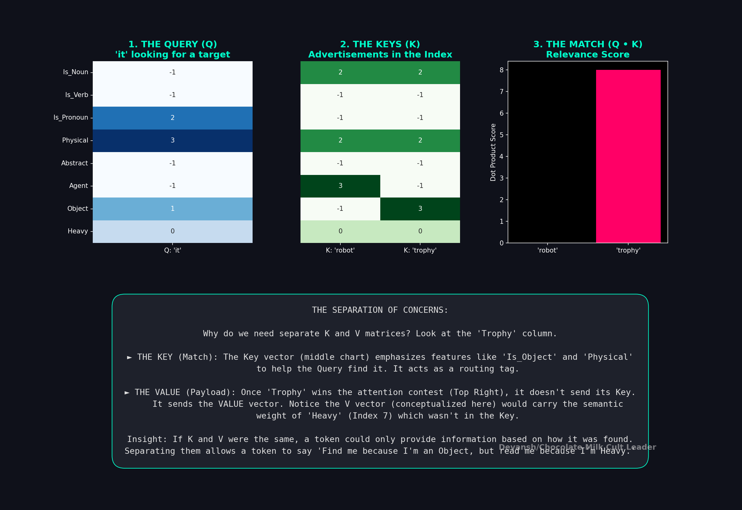
The transformer solves this by treating language like a dynamic search engine. Because one vector cannot simultaneously serve three distinct roles cleanly, it uses 3 different projections (vectors specialized for different things) —
The Query asks: What am I looking for?
The Key says: Here’s what I represent.
The Value says: Here’s the information I’ll give you if you choose me.
A good way to think about this is that the Key that makes a token findable and the Value contains the token’s actual payload, the same way a book’s title helps you find it, but the contents are what you actually read.
To give each token these three identities, we project our input matrix X three separate times (we multiply by 3 learnable weight matrices; training helps us improve the weights on these matrices):
Q = X* W_Q (what every token is looking for),
K = X* W_K (what every token advertises), and
V = X* W_V (what every token will provide).
This is our first real cost. Our system started with one headache, and ended up with 3 (perhaps our solutions reflect us more deeply than we realize; what does that tell us about the God/system that led to us?)
These weight matrices (W_Q, W_K, W_V) must be stored, loaded from memory, and multiplied for every token. We count the exact cost in Section 2, for now we must revert to a simpler question. What does this accomplish, exactly? That is what we will touch on next.
1.3 Finding Relevance: The Geometry of Meaning
Now each token has a query vector and every other token has a key vector. We need a way to measure: how relevant is token jj j to token ii i?
This is where dot products come in. Some of you might have seen the formulation and wondered why everything uses dot products to figure our relevance. I can go into the math, but I think that is mostly unneccesary. Instead, it’s better to understand why Dot Products are the right tool here by analyzing their behavior —
Two vectors pointing in the same direction yield a large positive dot product.
Orthogonal vectors yield zero. Precisely the behavior we would want from irrelevant ideas interacting with each other.
Vectors pointing in opposite directions yield a large negative value.
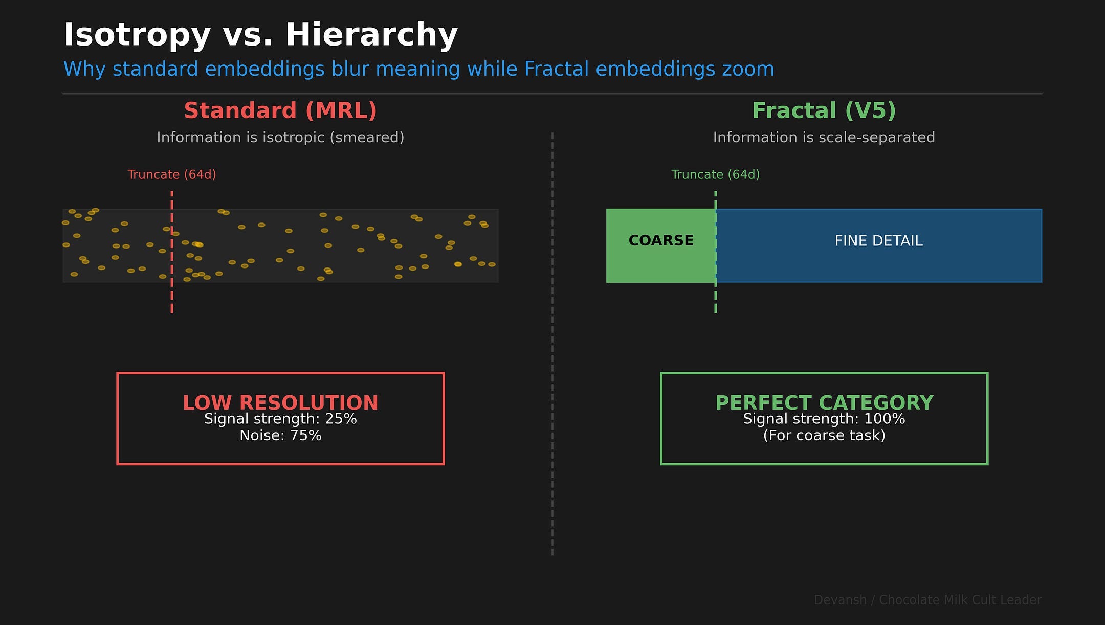
There’s a reason we’re adopting this framing. Understanding how each math tool behaves and why it plays a role in enforcing the behavior we desire is a great way to dip your feet into research. Playing with this framing will let you start exploring how you can build your own frontier modifications w/o needing a math degree or extreme credentials. For example, our work on Fractal embeddings didn’t start with deep math theory, but rather a simple observation: we needed a way to integrate hierarchies in embeddings. Everything else came downstream from that.
So if you’re struggling to understand the math/theory behind AI, it can be helpful to take a step back and understand what behavior a formula/particular will enforce and then contextualize that in the broader context of the topic. If you’re looking for a concrete guide on that specific skill, this article will be very useful to you.
During training, the model learns to arrange queries and keys so that tokens that *should* attend to each other end up pointing in similar directions in this shared space. A pronoun’s query vector gets pushed to align with the key vectors of plausible referents. A verb’s query aligns with subject keys. The entire attention mechanism is the model learning a geometry of relevance.
We compute this for all pairs at once with a single matrix multiplication: S = QK^T. The result is a giant n × n matrix of raw relevance scores. For a 4K context, that’s 4096 × 4096, roughly 16.8 million comparisons. This is where the famous quadratic cost comes from. It’s not an implementation detail; it’s the price of global context.
You may have heard that FlashAttention solves this. It’s critical to understand what it fixes and what it doesn’t. A naive implementation stores that full n × n matrix in the GPU’s high-bandwidth memory (HBM), which is slow. FlashAttention cleverly avoids this by computing attention in small blocks that fit in the GPU’s much faster on-chip SRAM, never materializing the full matrix in HBM. This dramatically speeds things up by optimizing memory access. But the number of mathematical operations remains exactly the same. The computation is still quadratic. FlashAttention is a brilliant engineering feat that makes better use of the hardware; it does not change the underlying math.
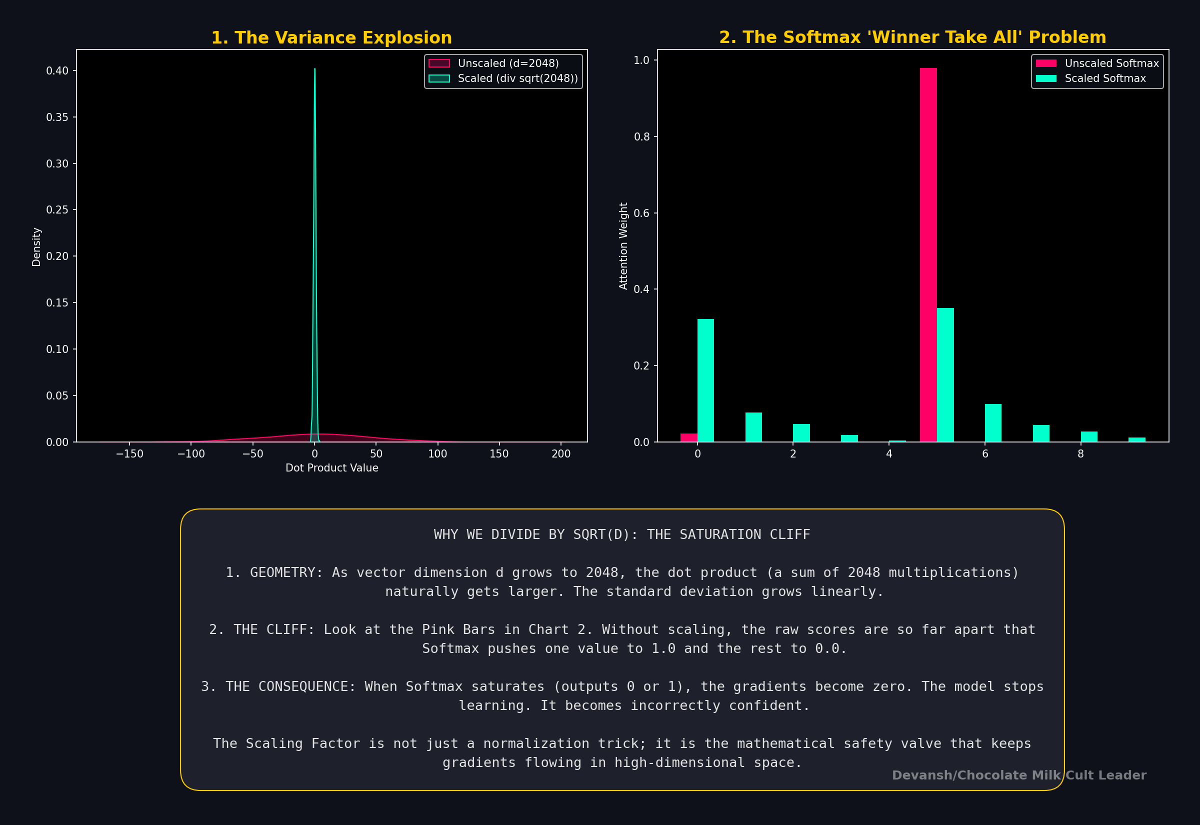
1.4: Making the Dot Products Stable
If we stopped at dot products, each token would get a list of raw scores. But raw scores don’t give you a stable weighting scheme. They can be arbitrarily large or small. To make things stable, we need two things:
Non-negativity (negative weight would mean “anti-use this token,” which destabilizes aggregation).
Normalization (the weights should sum to 1, so the scale of the output doesn’t explode). It also allows us to use each value as a “percentage”, making life much easier.
The second is very important. The dot product is a sum of products. As the dimension d_k grows, the variance of this sum also grows, linearly with d_k. For d_k=64, the raw scores can have a standard deviation of 8 (it will always be the square root of the dimensions). ]
Let’s look at how we make things happen.
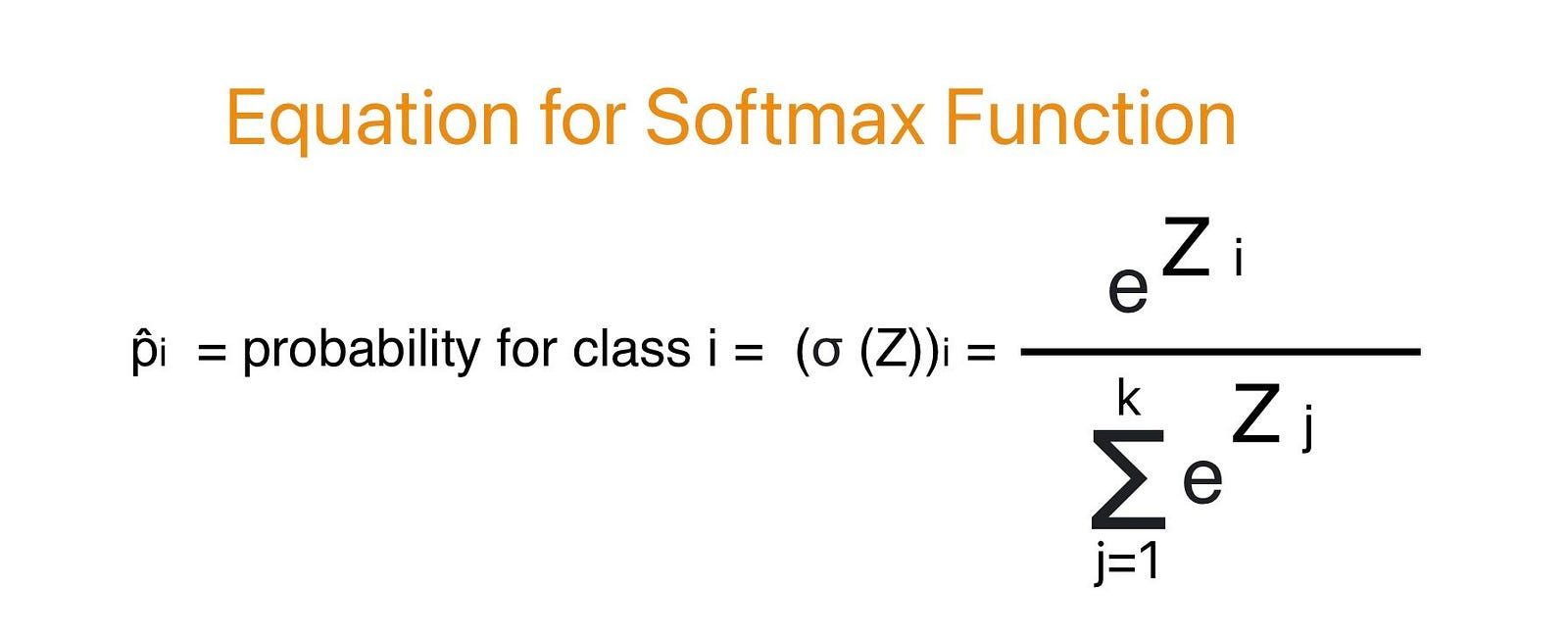
1.5 Softmax: Allocating a Fixed Budget
Now we need to turn our raw scores into a strict attention budget. Each token has 100% of its attention to give, and we need to decide how to allocate it. This requires converting our scores into a set of weights that are (a) all positive and (b) sum to exactly 1 for the reasons explained above.
This is the job of the softmax function:
The exponential exp(S_ij) guarantees all outputs are positive. It also exaggerates differences: a score of 10 vs 8 becomes ~7.4x the weight, not 1.25x( Without the exponential, a score of 10 vs 8 is just 10/8 = 1.25x the weight; with the exponential, it becomes e¹⁰ / e⁸ = e² ≈ 7.4x), turning a recommendation into a conviction. This bit is likely where we will see some pushback as we develop better ways to model uncertainty in our knowledge calculations.
Dividing by the sum forces the entire row to add up to 1, creating a perfect budget. The output, A, is our final attention map, a matrix where each row tells us the exact percentage of focus a token allocates to every other token.
1.6 Aggregation: Gathering the Information
We have our budget (A) and the information to be shared (V). The final step is to build a new, contextually-aware representation for each token: Output = AV.
This is a construction process. The new vector for “it” in our sentence is built by taking a weighted blend of all other tokens’ Value vectors. If its budget allocates 70% to “trophy” and 20% to “robot,” its new vector becomes a combination of their Value vectors. It has literally absorbed the semantic properties of the words it refers to, physically pulling its vector representation closer to theirs in high-dimensional space.
1.7 Multi-Head Attention: Specialists in Parallel
A single attention mechanism might learn to track, say, subject-verb agreement. But language requires tracking many relationships at once — syntactic, semantic, positional.
Multi-Head Attention runs h attention functions in parallel, each in its own learned subspace. Each head computes its own Attention(XW_Q^i, XW_K^i, XW_V^i), then the results are concatenated and projected back to the full model dimension with a learned output matrix W_O.
Think of each head as a specialist. One tracks syntax, another tracks semantics. The output projection W_O learns how to synthesize the findings of all these specialists. Mathematically, this relaxes a rank-bottleneck: a single head can only express a limited variety of attention patterns. Multiple heads allow for a much richer, higher-rank approximation of the ideal relevance map.
Dealing with multiple heads gets very expensive, which is where we will touch on the final innovation you need to know to really understand transformers.
1.8 Grouped Query Attention: An Economic Compromise
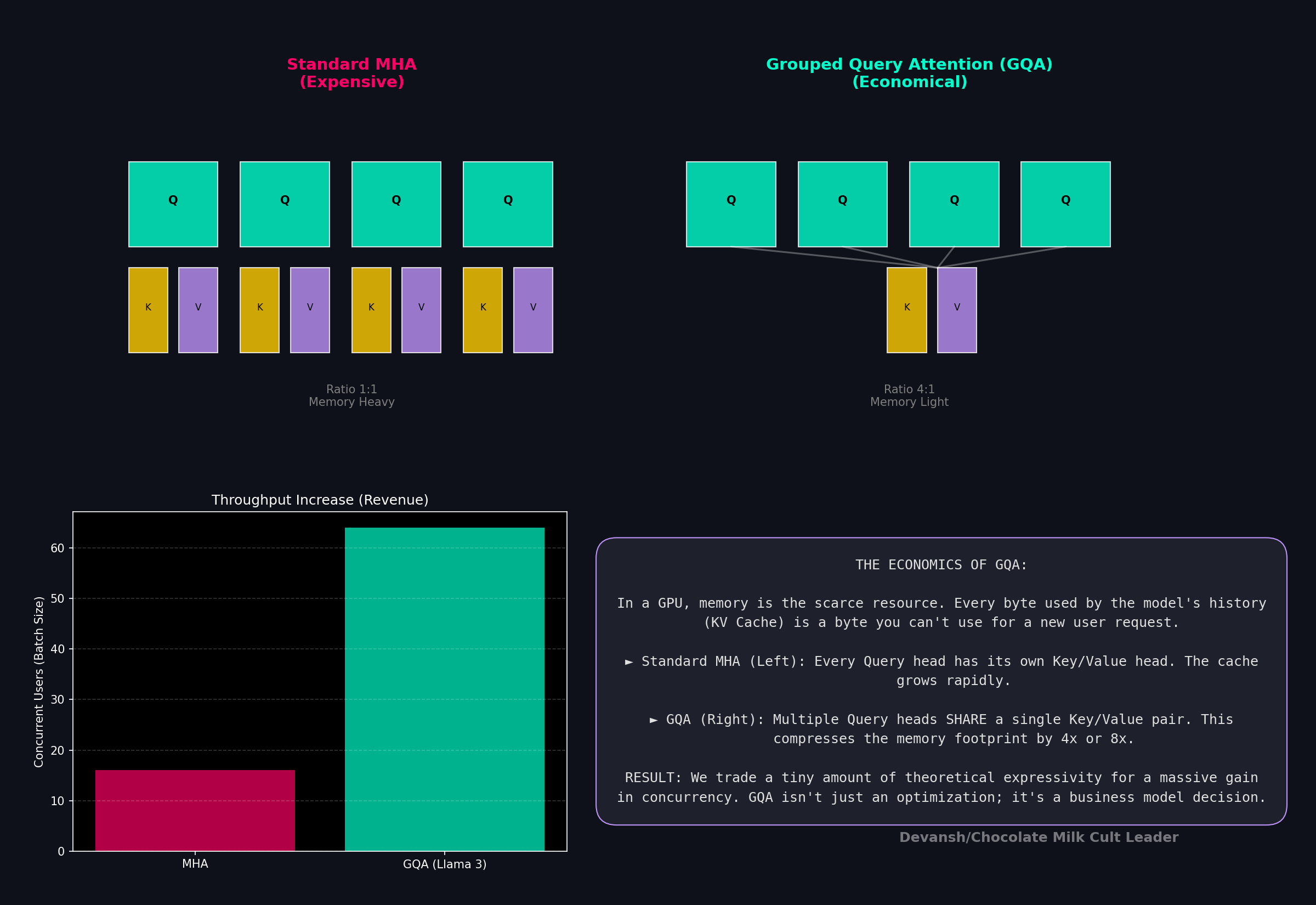
Every head in standard MHA has its own Key and Value. During generation, these are stored in a KV cache, which grows with every new token. This cache is the binding constraint on how many concurrent users a single GPU can serve. Every byte of KV cache for one user is a byte unavailable for another. This directly caps revenue per GPU.
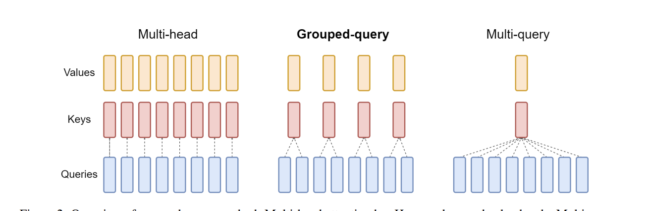
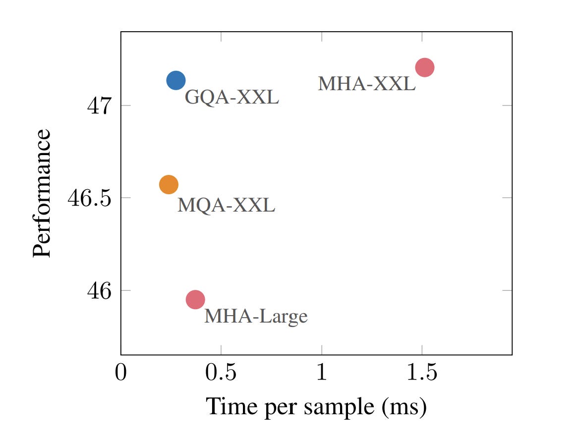
Grouped Query Attention (GQA) is a purely economic compromise. Instead of h KV heads, it uses a smaller number, g, and has multiple query heads share each KV pair. For Llama 3.2, 32 query heads share 8 KV heads, cutting the KV cache size by 4x. The quality loss is minimal, but the increase in concurrency is substantial. Every modern production model uses GQA because the memory savings translate directly into a lower cost per token.
If you can appreciate everything we’ve discussed, you now have a very strong working understanding of self-attention and why it uses the terms that it does. This puts us in a great place to discuss the costs of this damn thing.
2. How Much Does One Layer of Thought Cost
Every operation we described in Section 1 — projecting a query, calculating a score, aggregating a value — corresponds to a precise number of floating-point operations (FLOPs). FLOPs are the fundamental currency of compute. They determine how long a GPU is rented, how much electricity is burned, and ultimately, the base cost of every token you generate.
So let’s run the numbers to figure out exactly how many ops we’re running when you ask ChatGPT to draft Valentine’s Day notes for you.
A quick note on counting: a matrix multiply of an (a × b) matrix with a (b × c) matrix requires a × b × c multiply-add pairs. Each pair is 2 FLOPs (one multiply, one add). So the cost is 2abc. Remember this since it is the basis for a lot of the arithmetic.
Our variables:
n = sequence length
d = model dimension (2048 for a 1B model)
h = number of attention heads
d_k = d/h = dimension per head
2.1 The QKV Bill
Each of the three projections multiplies X (n × d) by a weight matrix (d × d), since all heads combined span d dimensions:
One projection = 2nd²
Three projections:
QKV total = 6nd²
This is a fixed cost. It doesn’t depend on how attention works internally — any mechanism that needs Q, K, and V pays this price. For a 1B model processing 4K tokens: 6 × 4096 × 204⁸² ≈ 103 billion FLOPs. Just to set up the search.
2.2 The Score Matrix
This is where we pay for global context. Each head computes Q times K-transposed: an (n × d_k) times (d_k × n) multiply.
Per head = 2n² × d_k
Across all h heads, and since h × d_k = d:
All heads = 2n²d
Notice the n². Double the context length, quadruple the cost of this step. At 4K context with d = 2048: about 68 billion FLOPs. At 32K: 4.4 trillion. This single operation is why long-context inference is expensive — and why it becomes the dominant cost as context grows.
2.3 Value Aggregation
Multiplying the attention weights (n × n) by the values (n × d_v) has the same structure:
Value aggregation = 2n²d
Same quadratic scaling. Same sensitivity to context length. The score computation and value aggregation together account for 4n²d FLOPs — the entire quadratic component of attention.
2.4 Output Projection
Each attention head produced its own output — an (n × d_k) matrix. With 32 heads and d_k = 64, that’s 32 separate (n × 64) results. These heads operated completely independently in their own subspaces. Head 3 has no idea what Head 17 found. We need to do something to bring all their insights together.
The first step is concatenation: stacking all 32 chunks of 64 dimensions side by side into one (n × 2048) matrix. No computation here; at this point the heads’ outputs are sitting next to each other but haven’t actually interacted.
The second step is where the interaction happens. The output projection W_O is a learned (d × d) weight matrix — (2048 × 2048) — that the concatenated result gets multiplied through. This is where the model learns how to synthesize the findings of different specialists. When one head found a syntactic subject and another found a semantic match, W_O learns how to combine those signals into something more useful than either alone. Without it, the heads’ findings are just glued together with no synthesis.
The concatenated output is an (n × d) matrix — n tokens, each with d dimensions. W_O is a (d × d) matrix. We’re multiplying (n × d) times (d × d). Using the rule from the top of the section — an (a × b) times (b × c) multiply costs 2abc — we get:
Output projection = 2nd²
2.5 Attention Total
We now have 6nd² for the three QKV projections + 2nd² for the output projection, 2n²d for the score matrix , and 2n²d for value aggregation. This gives us the cost of MHA as —
Attention FLOPs per layer = 8nd² + 4n²d
When n is small relative to d, the 8nd² projection terms dominate — you’re mostly paying for the linear algebra of setting up Q, K, V and recombining heads.
When n grows large, the 4n²d terms take over — you’re paying for the quadratic cost of every-token-looks-at-every-token.
The crossover happens at n = 2d. For d = 2048, that’s n = 4096. Below 4K tokens, projections dominate. Above 4K, attention dominates. As an interesting historical fact, this is why 4K was the standard context length for years (and is the still the context for some edge models). Beyond that threshold, the economics of attention change fundamentally.
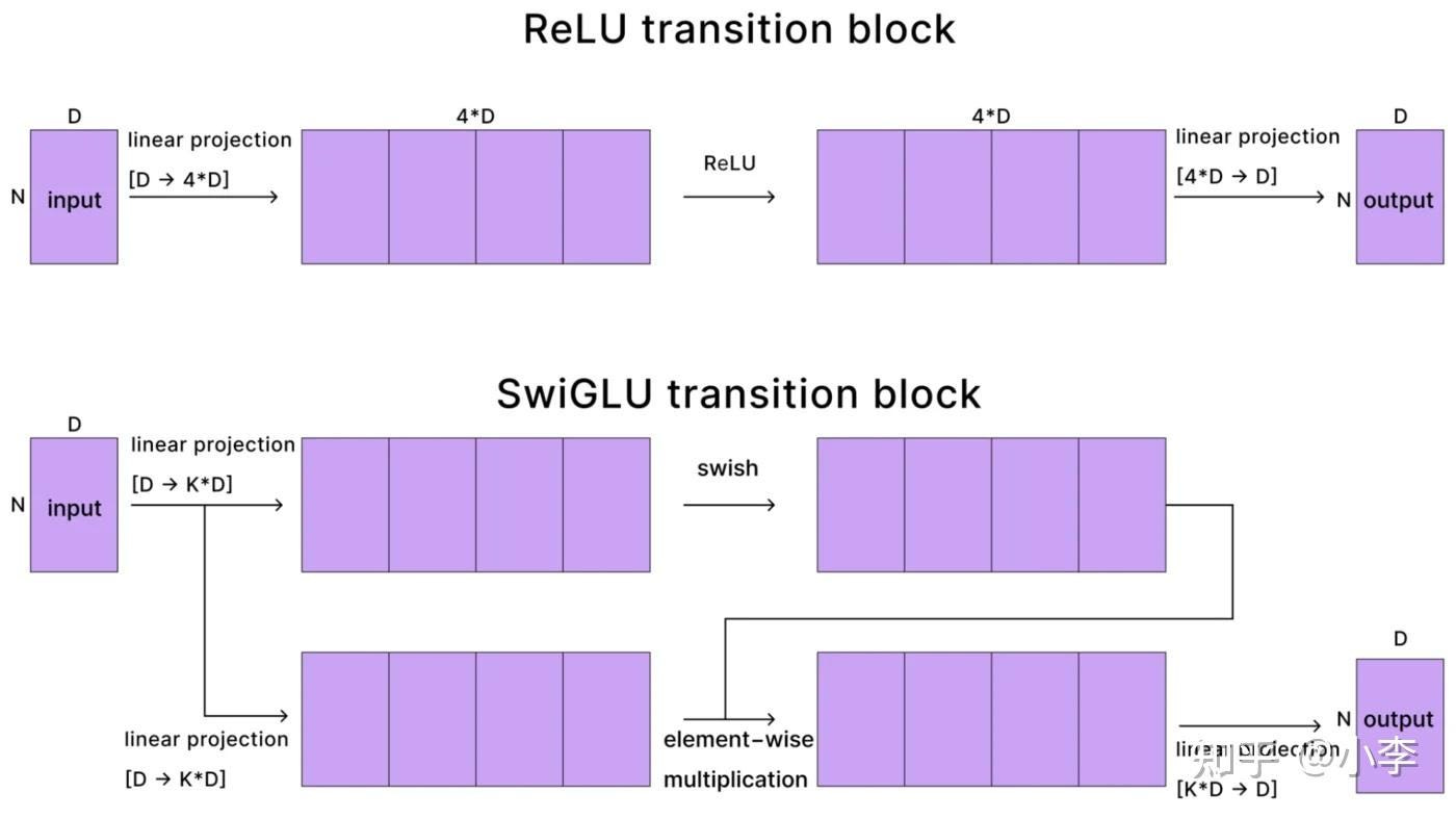
2.6 The MLP: The Other Half of the Bill
Attention gets all the headlines, but there’s an equally expensive component most people overlook: the MLP (feed-forward network; these days often a Mixture of Experts) that follows every attention block.
^^Image Credit to Sebastian Raschka, PhD (his work is great, check him out)
Attention moves information between tokens while the MLP transforms each token’s representation independently. Put another way, while attention decides what information to gather, the MLP decides what to do with it.
Modern transformers use a variant called SwiGLU. The classic MLP design uses two matrices that expand from d to 4d and back — each costing 8nd², totaling 16nd². SwiGLU uses three matrices with a slightly smaller expansion factor (8d/3 instead of 4d), but three times 16nd²/3 lands at the same total MLP FLOPs per layer = 16nd².
That’s twice the cost of the attention projections alone. The MLP is not the sideshow — it is half the bill. For a 1B model at 4K context, the MLP costs about 274 billion FLOPs per layer. More than the entire attention mechanism at that context length.
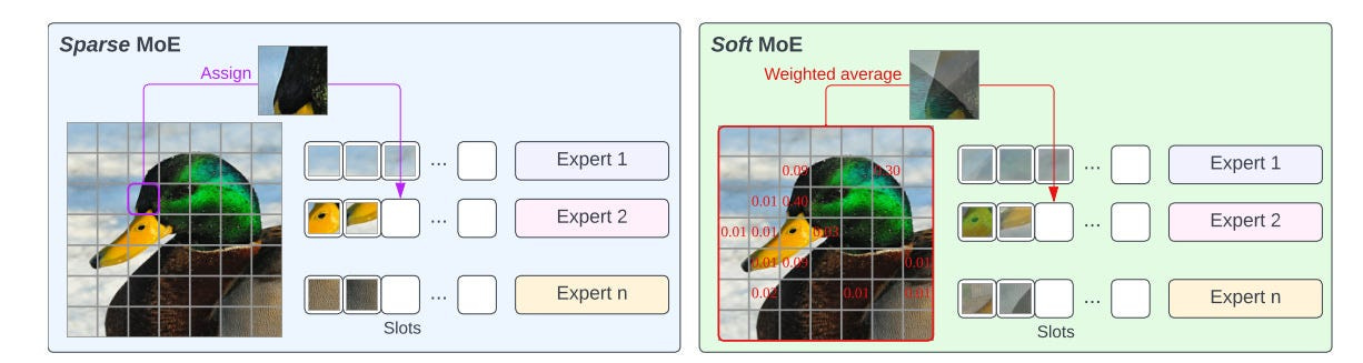
You may have heard of Mixture of Experts (MoE) as a way to make this cheaper. MoE replaces the single dense MLP with many smaller “expert” MLPs and a router that picks the top-k for each token. A model with 32 experts and top-4 routing has 32× the MLP parameters stored on disk, but each token only passes through 4 of them — so the active FLOPs per token drop dramatically. This is why Mixtral 8x7B has 47B total parameters but runs at roughly 13B speed. The catch: all those expert weights still need to be stored and loaded into memory, so MoE trades compute savings for a larger memory footprint.
It changes the FLOPs-per-token math significantly, but it does not change the memory bandwidth problem, which, as we’ll see in Section 4, is the actual bottleneck during generation. And for the purposes of this section, it also doesn’t change the costs of the actual active MLPs.
2.7 The Formula
One complete transformer layer:
Layer FLOPs = MLP FLOPs + Attention FLOPs= 8nd² + 4n²d + 16nd²= 24nd² + 4n²d
Every transformer model ever deployed runs some variant of this formula at every layer. We need only multiply by L layers for the full model costs.
Let’s make it concrete for a 1B-class model (d = 2048, L = 16):
At 1K context: the quadratic term is about 8% of total cost. The model spends almost all its compute on projections and the MLP.
At 4K context: the quadratic share rises to 25%. This is roughly the crossover zone — projections and attention are comparable.
At 32K context: the quadratic term is 73% of total. Most of the compute is now spent on the n × n attention matrix.
At 128K context: the quadratic term is 92%. Almost everything the model does is attention. Projections and MLP become rounding errors.
This is the fundamental economic tension of the transformer: short contexts are cheap because the d² terms dominate, and those scale linearly with n. Long contexts are expensive because the n² term takes over, and that scales quadratically. Every pricing model, every latency target, every hardware purchasing decision traces back to where a given workload falls on this curve.
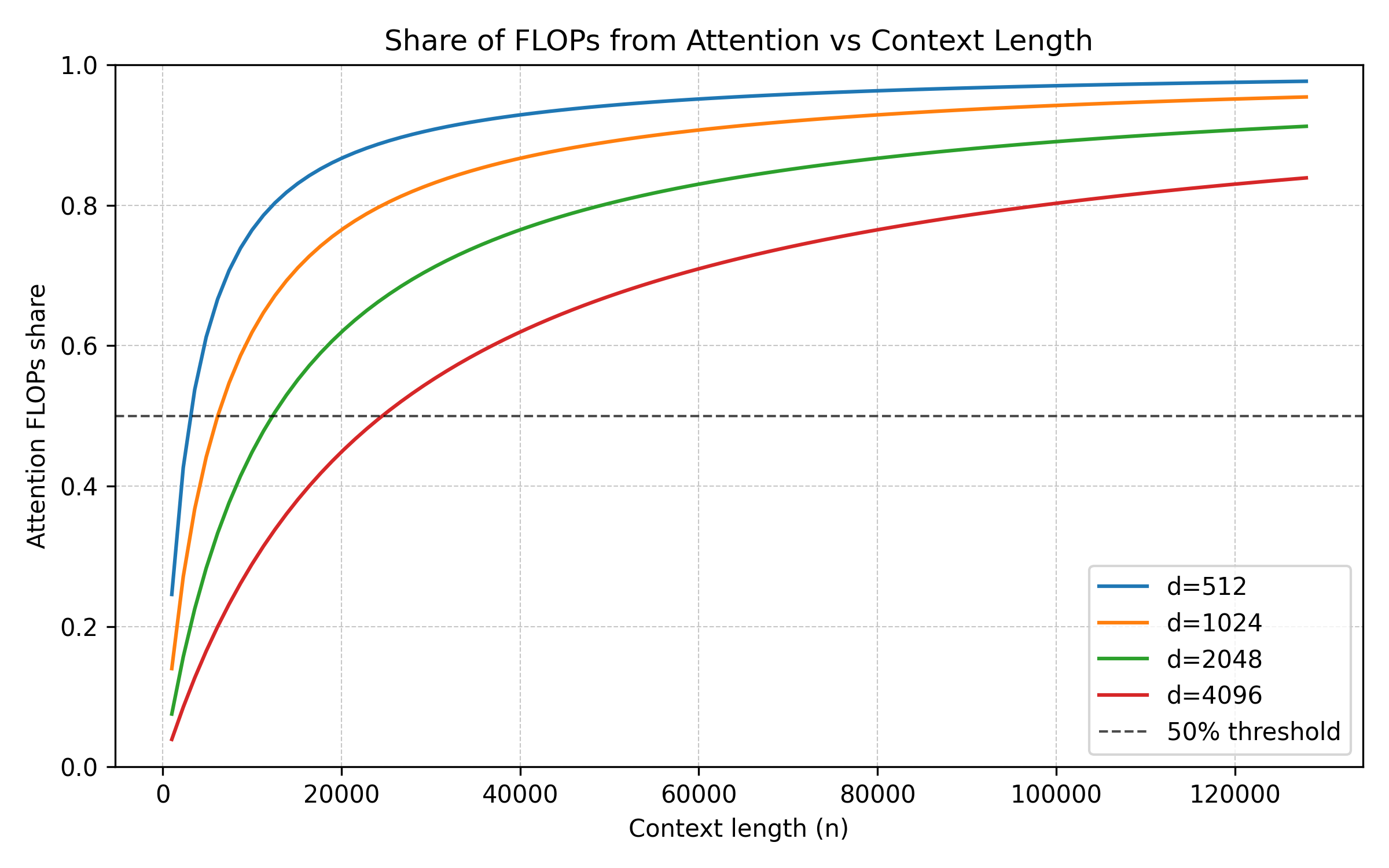
The formula also tells you where architectural innovation can actually help. The 24nd² term is mostly unavoidable — any model that processes tokens through weight matrices pays this. The 4n²d term is the target. Any architecture that reduces or eliminates the quadratic component — without destroying quality — fundamentally changes the cost structure. That’s what the entire alternative-architecture space is trying to do. We will do a follow-up deep dive exploring the work here in much more detail.
For now, we have our price tag. However, this is still a simplification. In reality, inference is really two things under the hood: prefill and decode . This formula behaves in radically different ways for each, with massive consequences for performance and cost.
So let’s break this down further.
3. Prefill vs Decode: Two Completely Different Machines
If you look at an API pricing page, you’ll see something strange: input tokens (what you send) are almost always cheaper than output tokens (what the model generates). Sometimes by a factor of 3 or 4.
Why? The model is doing the exact same math for both. It’s the same weights, the same layers, the same attention mechanism. So why is reading a book so much cheaper than writing one?
The answer lies in hardware physics. Inference isn’t one process; it’s two completely different workloads that happen to share a neural network.
3.1 Prefill: Processing the Prompt
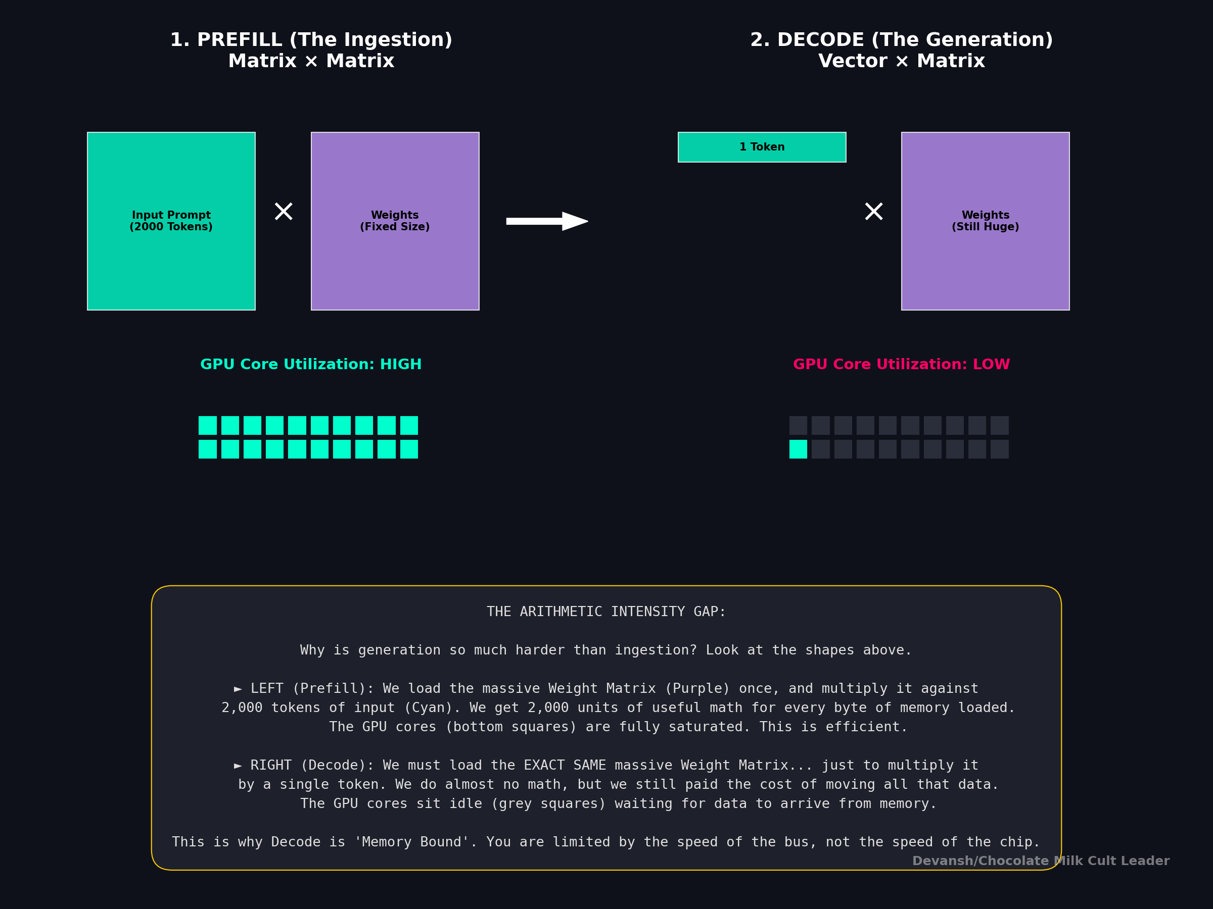
When your prompt arrives — say, 2,000 tokens of context — the model processes all of them at once. Every token in the prompt is known ahead of time, so the model can compute Q, K, and V for all 2,000 tokens in a single batched matrix multiplication.
This is matrix times matrix arithmetic. X (2000 × 2048) multiplied by W_Q (2048 × 2048). Both operands are large. The GPU’s thousands of cores can all work in parallel because there’s enough data to keep them fed.
The key concept to understand here is arithmetic intensity — the ratio of compute operations to bytes of memory moved. It tells you whether your hardware is spending its time doing useful math or sitting idle waiting for data.
We also need to understand bytes per parameter (B_p) — how many bytes each number in the model takes to store. Standard FP16 precision uses 2 bytes per number. INT8 (a common quantization format) uses 1. INT4 uses half a byte. This matters because it determines how much data the GPU physically moves through its memory bus for each operation.
For the QKV projections during prefill:
FLOPs: 2 × n × d × d = 2nd² per projection
Bytes loaded from memory: roughly d² × B_p (the weight matrix dominates)
Arithmetic intensity: 2nd² / (d² × B_p) = 2n / B_p
That ratio grows with n. More tokens in the prompt means more useful compute per byte of memory loaded. At n = 4096 with FP16 (B_p = 2): arithmetic intensity is 4096. That means 4096 FLOPs of useful work for every byte moved — the GPU’s compute cores are saturated. This is a good situation. The hardware is doing what it was designed to do.
For the attention score computation (Q times K-transposed), arithmetic intensity is n / B_p — lower than the projections but still grows with sequence length. At any reasonable context length, both operations are firmly compute-bound.
The bottom line: prefill is compute-bound. The GPU is limited by how fast it can multiply, not how fast it can read from memory. This is the regime GPUs were designed for — big batches of parallel math, keeping every core occupied.
3.2 Decode: Generating One Token at a Time
Now the model has processed the prompt and needs to generate a response. Here’s the critical difference: it generates one token at a time. Each new token depends on the one before it so you can’t parallelize this. The model produces token 1 of the response, then uses that to produce token 2, then token 3, and so on.
This means every step is matrix times vector. The new token’s embedding (1 × d) gets multiplied by the weight matrix (d × d). One row times a full matrix. Every single step.
The arithmetic intensity collapses:
FLOPs: 2 × 1 × d × d = 2d² per projection
Bytes loaded: d² × B_p (still loading the full weight matrix — for a single token)
Arithmetic intensity: 2d² / (d² × B_p) = 2 / B_p
For FP16: arithmetic intensity = 1. For INT8: 2. For INT4: 4.
Compare this to prefill’s arithmetic intensity of thousands. During decode, the ratio is a single-digit number independent of everything — model size, context length, architecture. It doesn’t matter if you’re running GPT-4 or a 350M model. Every single weight in the model gets loaded from memory to process one token, and the compute done with each weight is trivial.
This is what it means to be memory-bound. The compute cores are idle almost all the time, waiting for data to arrive from memory. You could double the FLOPs on the chip, and decode speed would barely change — because the bottleneck isn’t math, it’s the speed of the memory bus.
3.3 The Same Formula, Two Different Worlds
Our layer cost formula is 24nd² + 4n²d. But n means something different in each regime:
During prefill, n is the full prompt length. The 4n²d term is large (quadratic in context), but the GPU is compute-bound and well-utilized. The formula predicts total work, and the GPU chews through it efficiently.
During decode, n = 1 for the new token. The 4n²d attention term collapses — but not entirely, because the model still reads the full KV cache of all previous tokens to compute attention scores. The real cost per decode step is dominated by loading model weights plus reading the growing KV cache, not by multiply-add operations. The formula tells you the FLOPs, but the actual wall-clock time is governed by memory bandwidth.
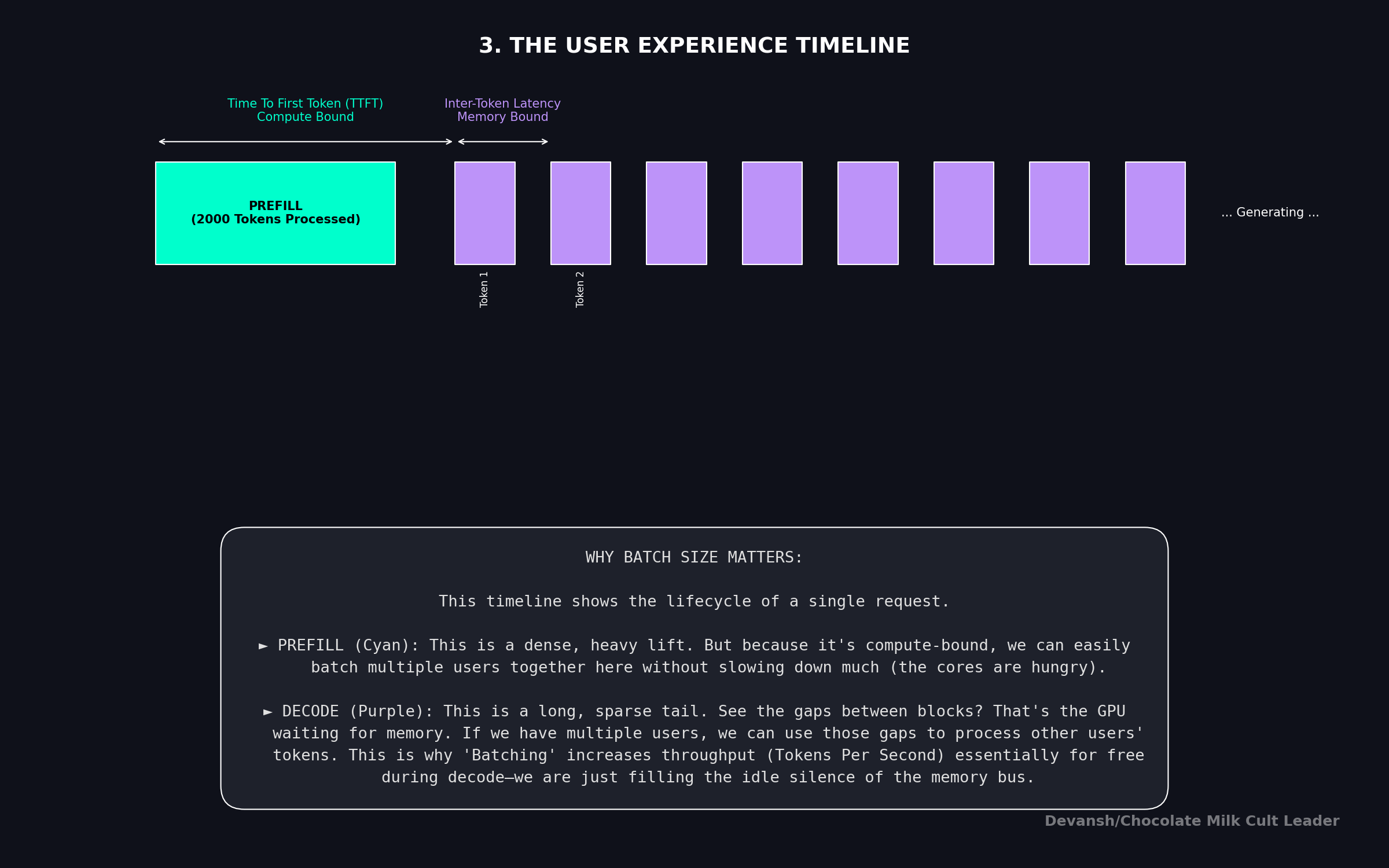
This is why “inference” is a misleading single word. Prefill performance is measured in total tokens processed per second — how fast you can ingest a prompt. Decode performance is measured in output tokens per second — how fast you can generate. They have different bottlenecks, different scaling properties, and different optimization strategies.
3.4 Why This Matters for Cost
The prefill/decode split has direct economic consequences:
Time-to-first-token (TTFT) is dominated by prefill. A long prompt means a long wait before the first response token appears. This is compute-bound — you can speed it up by adding more GPU compute or by reducing the FLOPs in the model architecture.
Tokens-per-second (TPS) during generation is dominated by decode. This is memory-bound — adding more compute doesn’t help. You speed it up by increasing memory bandwidth (more expensive hardware), reducing model size (fewer bytes to load per step), or shrinking the KV cache (less data to read per step).
These are different bottlenecks requiring different solutions. A provider optimizing for TTFT buys more compute. A provider optimizing for TPS buys more bandwidth. Conflating the two leads to bad purchasing decisions — and this happens constantly because most infrastructure discussions don’t distinguish the regimes.
The split also determines pricing structures. Input tokens (which go through prefill) and output tokens (which go through decode) have fundamentally different hardware profiles. This is why every major API provider charges different rates for input vs output tokens — it’s not arbitrary, it’s physics. Output tokens are more expensive because decode has worse hardware utilization. You’re paying for a GPU that’s mostly waiting.
3.5 The Implication for Architecture
As mentioned earlier, during decode — the bottleneck regime, the one that determines generation speed and output cost — the binding constraint is memory bandwidth. Specifically:
How many bytes of model weights must be loaded per token
How many bytes of KV cache must be read per token
Any architecture that reduces either of these numbers directly speeds up generation and reduces cost.
The KV cache is the variable that grows. Model weights are fixed after deployment. But the KV cache grows with every token generated, making decode progressively slower and more expensive over long outputs. In Section 5 we will derive exactly how fast it grows — and the hard ceiling it puts on GPU concurrency.
First, though, we need to formalize the relationship between compute, memory bandwidth, and utilization. That is the roofline model, and it is what makes the prefill/decode split rigorous instead of hand-wavy.
4. The Roofline: Why Hardware Sits Idle While You Pay For It
In Section 3, we said prefill is compute-bound and decode is memory-bound. Let’s prove them — and show that this isn’t a quirk of current hardware but rather a structural mismatch between what decode needs and what chips provide. Ultimately, no amount of hardware scaling fixes it.
4.1 Every Chip Has Two Speeds
Every processor — GPU, CPU, NPU, whatever — has two independent performance limits:
Peak compute: how many operations per second the chip can perform. An H100 does about 989 trillion FLOPs per second (TFLOPS) at FP16. A Snapdragon 8 Elite phone CPU does maybe 50 billion (GFLOPS). That’s a 20,000× gap.
Memory bandwidth: how many bytes per second the chip can move between memory and compute cores. An H100 moves 3,350 GB/s. A Snapdragon 8 Elite moves about 51 GB/s. That’s a 66× gap.
Notice something: the compute gap (20,000×) is vastly larger than the bandwidth gap (66×). GPUs are disproportionately good at math compared to how fast they can feed data to the math units. This imbalance is the entire story.
4.2 The Roofline
The roofline model asks a simple question: for a given operation, which limit does the chip hit first?
If the operation does a lot of math per byte of data moved, compute is the bottleneck. The chip’s cores are maxed out and memory bandwidth has spare capacity. This is compute-bound — the good case.
If the operation does very little math per byte of data moved, memory bandwidth is the bottleneck. The chip’s memory bus is maxed out and most cores sit idle. This is memory-bound — the expensive case, because you’re paying for a chip that’s mostly waiting.
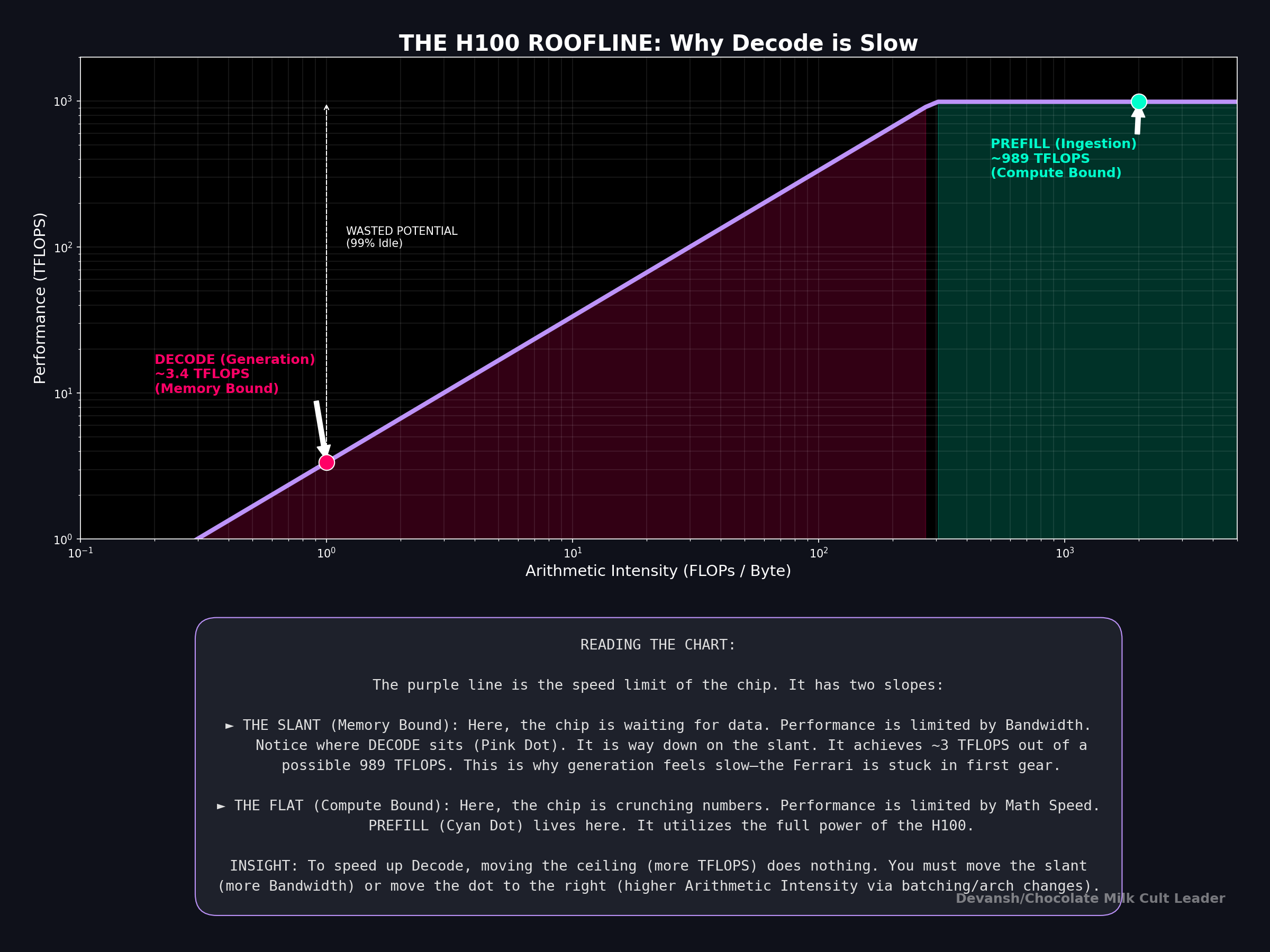
The dividing line is the chip’s compute-to-bandwidth ratio:
H100: 989 TFLOPS / 3,350 GB/s ≈ 295 FLOPs per byte
A100: 312 TFLOPS / 2,039 GB/s ≈ 153 FLOPs per byte
Snapdragon 8 Elite CPU: ~50 GFLOPS / 51 GB/s ≈ ~1 FLOP per byte
If your operation’s arithmetic intensity (FLOPs per byte, from Section 3) is above this ratio, you’re compute-bound. If it’s below, you’re memory-bound.
The actual performance you get can be quantified as follows:
Performance = the lower of (peak compute) or (bandwidth × arithmetic intensity)
That’s the roofline. Performance rises linearly with arithmetic intensity until you hit the peak compute ceiling, then flattens. You’re always limited by whichever resource runs out first.
4.3 Prefill Hits the Roof
We showed in Section 3 that prefill’s arithmetic intensity for QKV projections is 2n / B_p. At n = 4096 with FP16: that’s 4096 FLOPs per byte.
On an H100, the threshold is 295. 4096 >> 295. So we may infer that Prefill is deep into compute-bound territory. The GPU’s memory bus could be 10× slower and prefill performance wouldn’t change. All that matters is how fast the chip can multiply.
This is why GPUs are good at prefill. Their entire design — thousands of cores, massive parallelism, tensor cores — is built for compute-bound workloads. Prefill is the workload they were made for.

4.4 Decode Hits the Floor
Decode’s arithmetic intensity is 2 / B_p. At FP16: that’s 1 FLOP per byte. At INT4 (the most aggressive common quantization): 4 FLOPs per byte.
On an H100, the threshold is 295. We’re at 1–4. The chip is running at roughly 1% of its theoretical peak during decode. 99% of the compute silicon is idle, doing nothing, while the memory bus works as fast as it can to shuttle weight matrices to the few active cores.
This is the central insight of the roofline applied to LLM inference: during the phase that actually generates text — the part the user is waiting for, the part that determines tokens-per-second — the most expensive AI chip in the world is wasting 99% of its capability.
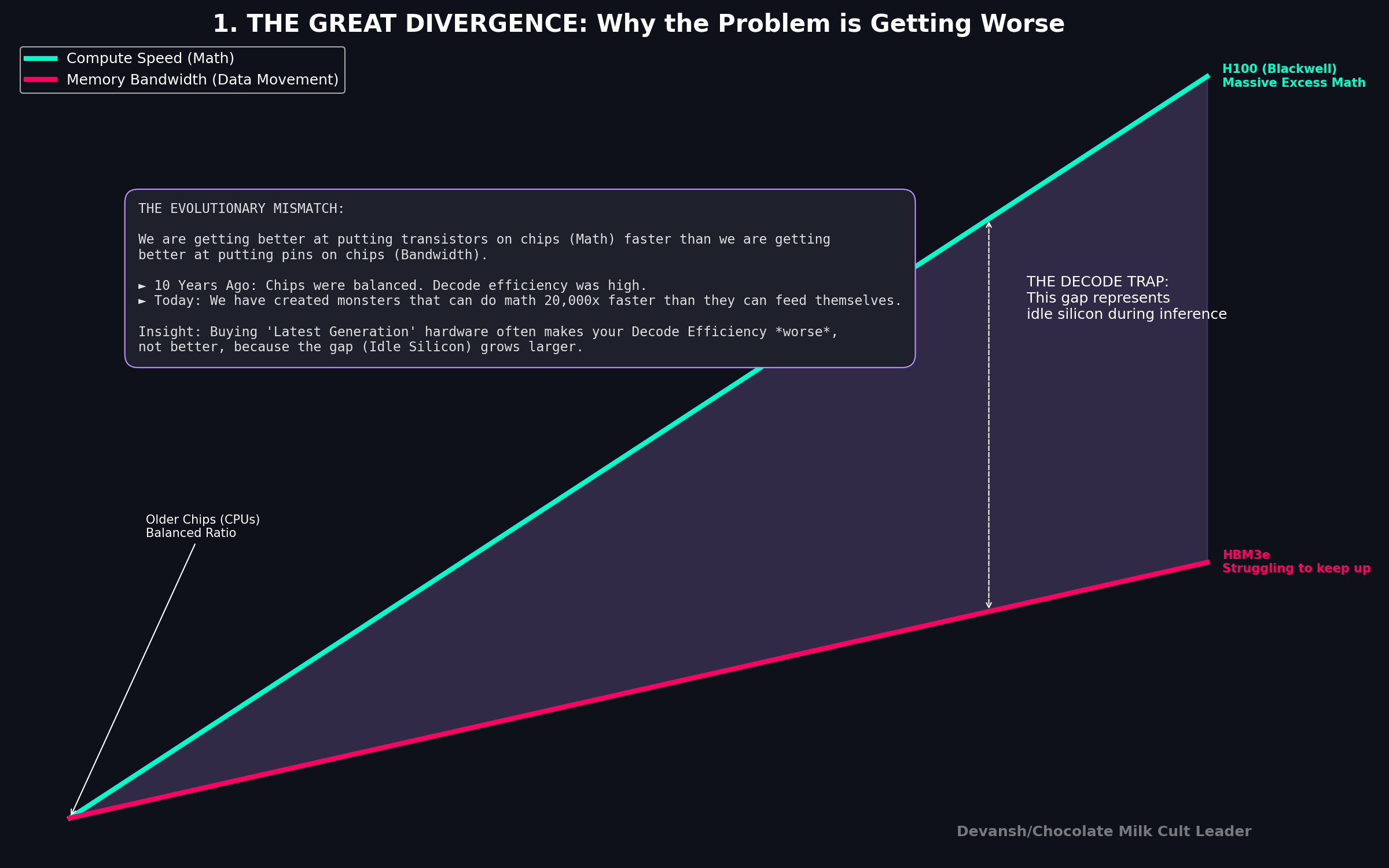
And this is not fixable by buying bigger hardware. Doubling the H100’s compute to 2000 TFLOPS would change nothing — decode would still be memory-bound. You’d need to double memory bandwidth, which is a far harder engineering problem (it’s limited by physics: the number of memory pins, signaling speed, power per pin).
This is exactly why inference-specific chips are emerging. Groq’s LPU uses massive on-chip SRAM to get bandwidth far above what standard HBM provides. Cerebras uses wafer-scale silicon with distributed memory. Etched is building transformer-specific ASICs. They’re all attacking the same roofline problem: pushing the compute-to-bandwidth ratio down so that decode lands closer to compute-bound territory. The tradeoff is that these chips sacrifice training capability — which needs NVIDIA’s raw FLOPS — to specialize for the memory-bandwidth bottleneck that dominates inference. NVIDIA keeps the training market. The inference chip startups are betting that the decode problem is large enough to sustain its own silicon ecosystem. This is a phenomenon we broke down in exhaustive depth (including modeling the ROI of different ASICs) over here, so read it if you’re interested.
4.5 What the Roofline Looks Like on a Phone
On a Snapdragon 8 Elite CPU, the compute-to-bandwidth ratio is about 1 FLOP per byte. Decode’s arithmetic intensity at INT4 is 4. So decode is actually compute-bound on a phone CPU — but only because the CPU is so slow that even the limited bandwidth can feed it fast enough.
Take a second to appreciate this switch. On a GPU, you have massive compute being starved by bandwidth. On a phone CPU, you have a tiny compute being barely fed by a tiny bandwidth. The experience is slow for a different reason — raw compute is the very low ceiling
Prefill on a phone is also compute-bound, but at a much lower throughput. A prompt that an H100 processes in 10ms might take a phone CPU 2–3 seconds. The user feels this as the time-to-first-token lag.
The implication: on-device models need to be architecturally smaller, not just quantized smaller. You can INT4-quantize a 7B model to fit in phone memory, but the compute required per token is still 7B-class. The only way to make it fast on a phone CPU is fewer parameters, which means the architecture itself needs to extract more quality per parameter. One of the reasons I’m writing this article is to give you an appreciation of the ecosystem that new entrants like Liquid AI are trying to disrupt by attacking these very angles.
4.6 The Roofline Determines Your Optimization Strategy
Once you know which side of the roofline you’re on, you know what to optimize:
Compute-bound (prefill, large batches): Buy more FLOPs. Use tensor cores. Increase parallelism. This is the problem NVIDIA has solved brilliantly — just add more cores.
Memory-bound (decode, batch=1): Buy more bandwidth. Or move fewer bytes. This means: smaller models (fewer weight bytes to load), aggressive quantization (fewer bytes per weight), smaller KV caches (fewer bytes to read per step), or architectures that avoid storing and reading KV caches entirely.
The entire alternative-architecture space — state space models, linear attention, convolution-based models — can be understood through this lens. They’re all trying to change the bytes-per-step equation during decode. The ones that succeed do so by replacing the KV cache with something smaller or eliminating it, directly attacking the memory-bound bottleneck that the roofline says is unfixable by compute scaling alone.
So everything seems like it boils down to the cache, doesn’t it?
That’s not a coincidence. If you strip away all the abstractions, the real bottleneck during generation is simple: How many bytes of weights and KV cache must be moved per token?
This is due to the fundamental tension of serving LLMs:
To make the GPU efficient, you need high concurrency (large batch size) so we can benefit from batching.
To run high concurrency, you need massive memory for the KV cache.
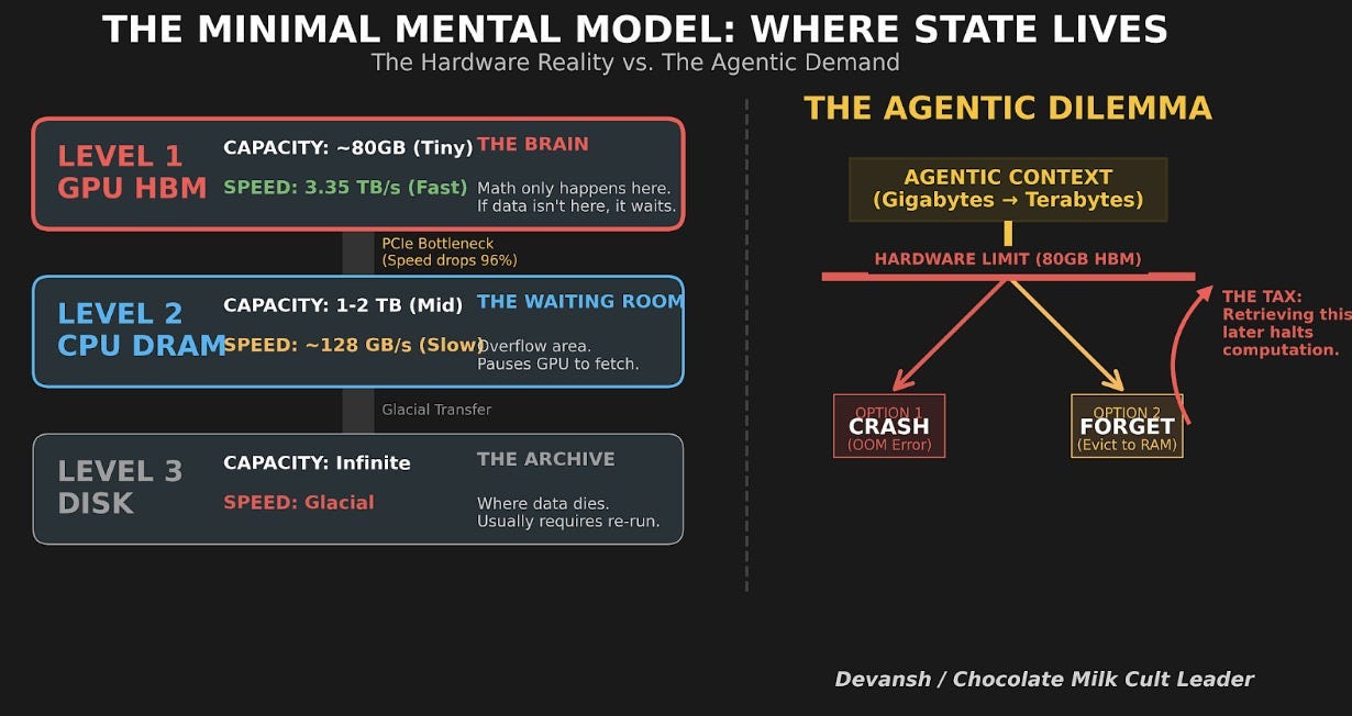
But GPU memory is finite (80GB on an H100).
Eventually, you run out of memory before you run out of compute. The KV cache fills up the VRAM, capping your batch size, forcing you back into the memory-bound regime, and killing your unit economics.
This is the Memory Wall. And in the next section, we will calculate exactly when you hit it.
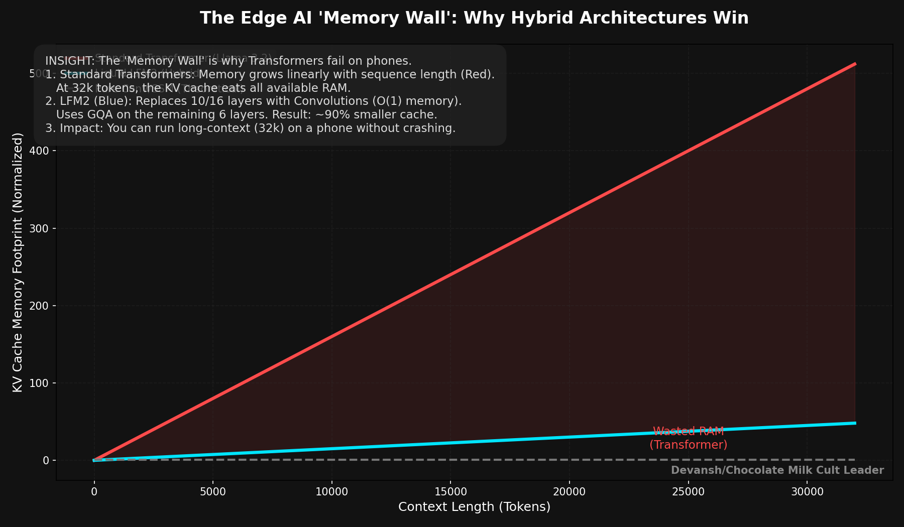
5. The KV Cache: The Tax That Grows With Every Token
In Section 3 we said the KV cache is the variable that grows during decode. In Section 4 we showed decode is memory-bound — the cache directly competes for the resource that’s already the bottleneck. Now we put exact numbers on how bad this gets.
5.1 Why the Cache Exists
During decode, the model generates one token at a time. Each new token needs to attend to every previous token. Computing attention for token 501 requires the key and value vectors of all 500 tokens before it.
Without caching, the model would recompute K and V for every previous token at every step. Token 501 reprojects tokens 1 through 500 through W_K and W_V from scratch — work already done at steps 1, 2, 3, all the way through 500. Token 502 does it all again, plus one more. Redundant compute, growing quadratically.
The KV cache kills this redundancy. Each time the model computes a new token’s key and value vectors, it appends them to a running cache. Next step, it only computes K and V for the new token and reads the rest. Quadratic recomputation becomes a linear read.
The tradeoff: that cache lives in memory. And it grows with every single token generated.
5.2 The Exact Memory Formula
Each attention layer stores one key vector and one value vector per token. Each vector has d_k dimensions (64 for most models). The cache stores these across every layer, for every token so far.
KV cache size = 2 × L_attn × g × d_k × n × B_p
The pieces: 2 (keys + values), L_attn (attention layers), g (KV heads — 8 for GQA models like Llama 3.2), d_k (dimension per head, often 64), n (current sequence length — the thing that grows), B_p (bytes per parameter, 1 for INT8).
Everything except n is a constant. That means the growth rate per token is fixed:
Bytes per new token = 2 × L_attn × g × d_k × B_p
Every token adds this exact amount. Doesn’t matter what the token is. Doesn’t matter what came before it. There will be a flat tax on generation.
5.3 Real Numbers
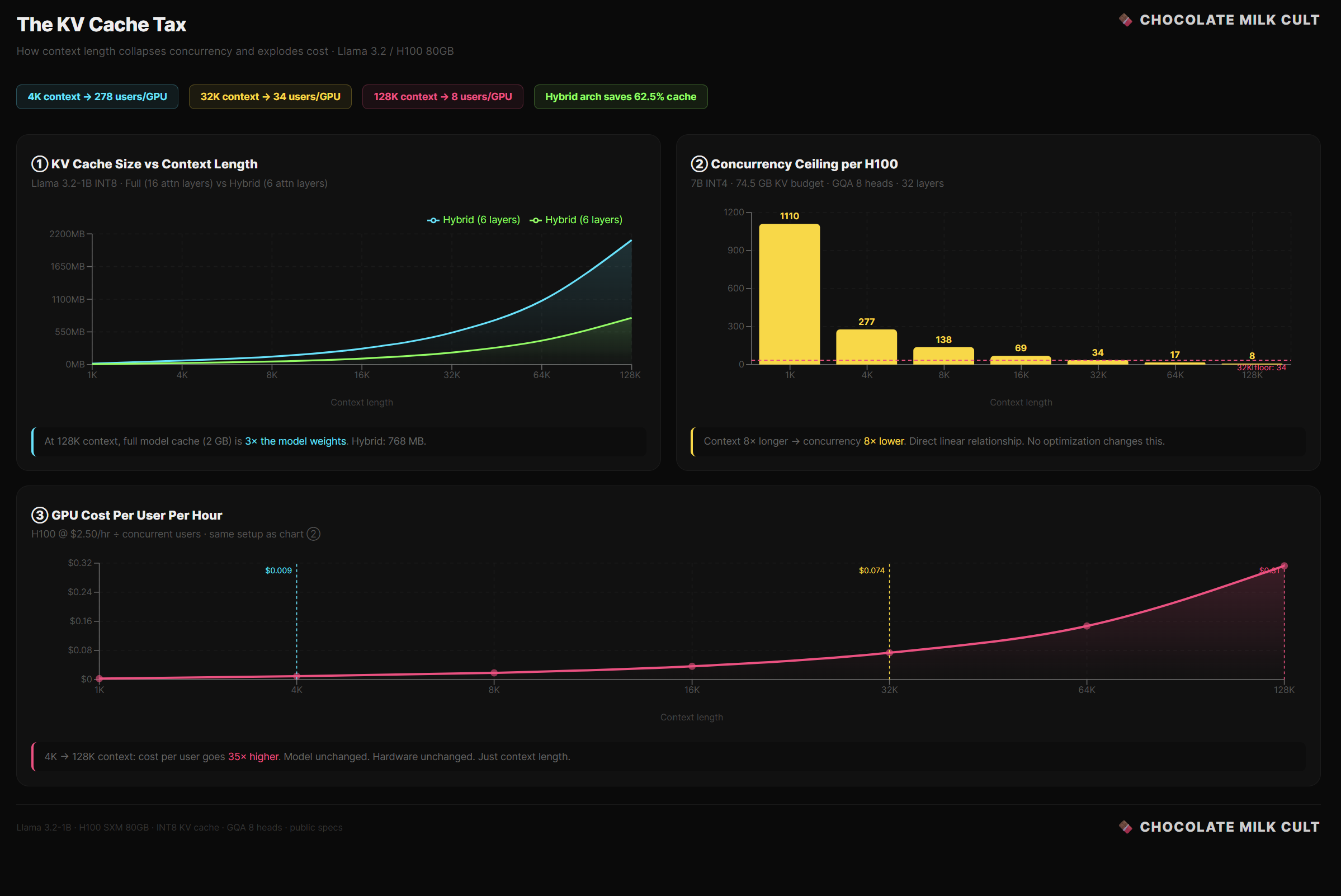
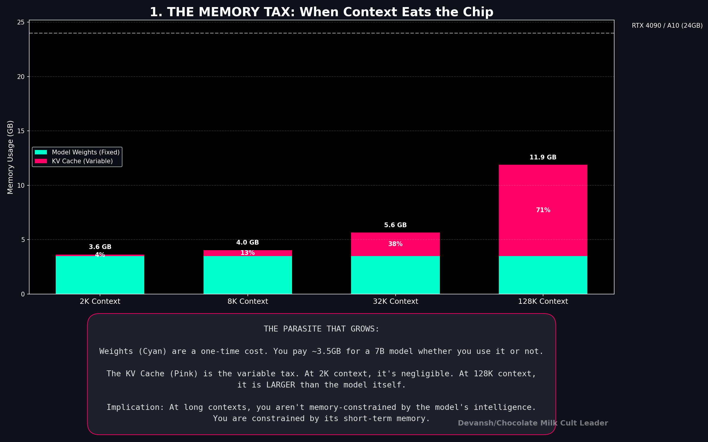
Take a 1B — pure transformer, 16 attention layers, 8 KV heads, d_k = 64, INT8:
Bytes per token: 2 × 16 × 8 × 64 × 1 = 16,384 bytes. Roughly 16 KB per token.
At 4K context: 67 MB. At 32K: 512 MB. At 128K: 2 GB.
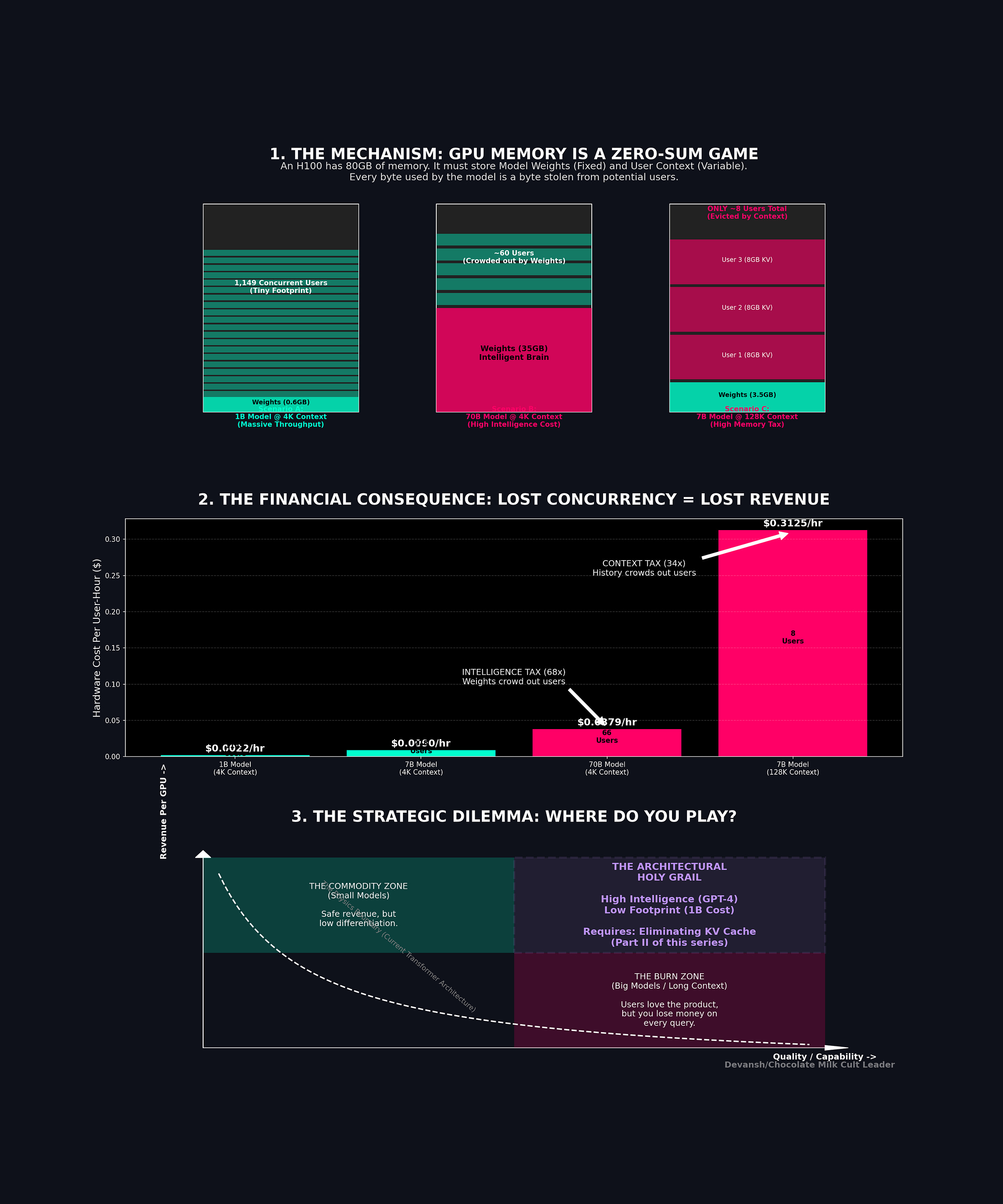
Sit with that 32K number for a second. The KV cache at 512 MB is approaching the model weights themselves (~600 MB at INT4). At 128K, the cache is more than 3× the weights. The thing that stores context has become larger than the thing that does the thinking.
Now swap in a hybrid architecture — say, only 6 attention layers instead of 16, the other 10 replaced by something that doesn’t need a cache:
Bytes per token: 2 × 6 × 8 × 64 × 1 = 6,144 bytes. About 6 KB.
At 32K: 192 MB instead of 512 MB. That’s 320 MB freed up. At 128K: 768 MB instead of 2 GB.
The reduction is exactly proportional to the fraction of layers you replaced — which is why hybrid architectures matter so much for the economics we’re about to derive.
5.4 The Memory Budget on a GPU
An H100 has 80 GB of HBM. Not all of it is yours to play with. First we have to handle the weights, which are a fixed cost:
A 70B model at FP16 eats ~140 GB (multi-GPU territory).
A 7B at INT4: ~3.5 GB.
A 1B at INT4: ~600 MB.
Then there’s activations — temporary, typically 50–200 MB. Framework overhead — CUDA context, memory allocator, scheduling buffers — another 1–2 GB.
What’s left is your KV cache budget. The pool is divided among every user talking to the model at the same time. For a 7B model at INT4 on an H100, that’s roughly 74.5 GB.
5.5 The Concurrency Ceiling
Each concurrent user needs their own KV cache. You can’t share contexts between people having different conversations (although that would be pretty fun to see).
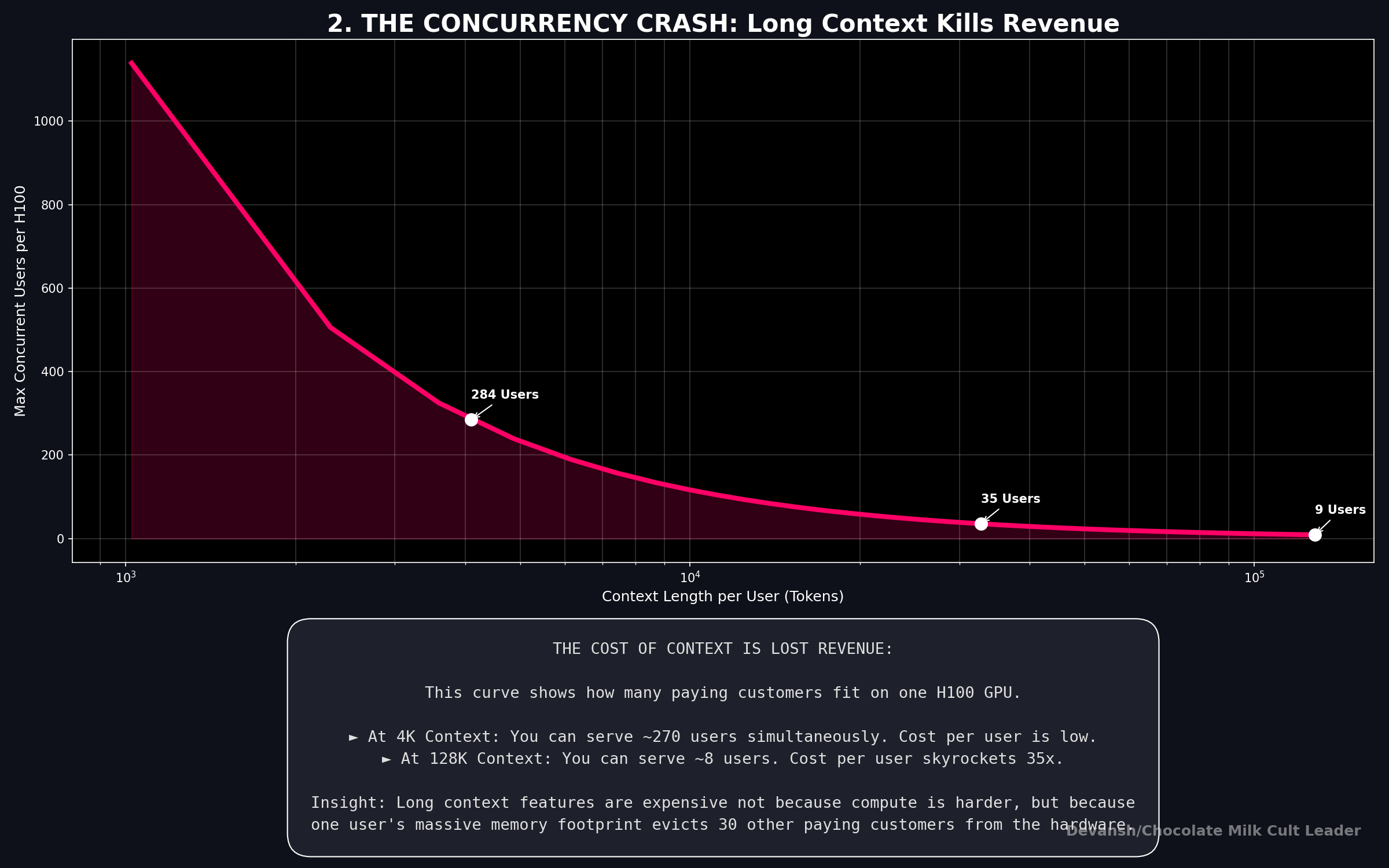
A 7B model with GQA, 8 KV heads, 32 layers, d_k = 128, INT8.
At 4K context, each session costs 268 MB.
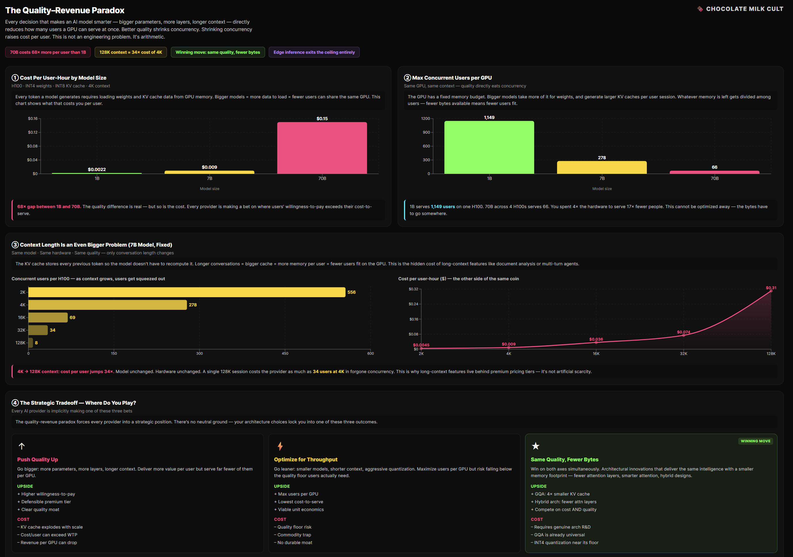
Divide 74.5 GB by 268 MB: 278 users per GPU.
At 32K context, each session costs 2.1 GB. With the same division, we now have 34 users per GPU.
Context went up 8×. Concurrency dropped 8×. It’s a direct linear relationship: Double the context, halve the users. No optimization changes this. The bytes have to live somewhere.
At 128K: ~8 users per GPU. You spent $30,000+ on a chip that serves 8 people at once.
5.6 What This Costs
An H100 rents for roughly $2.50/hour.
If you’re serving 278 concurrent users at 4K context, your per-user GPU cost is $2.50 / 278 ≈ $0.009/hour per user. Tight, but potentially viable.
At 32K context with 34 concurrent users: $2.50 / 34 ≈ $0.074/hour per user. Eight times more expensive, purely because context is 8× longer and concurrency dropped proportionally.
At 128K context with 8 users: $2.50 / 8 = $0.31/hour per user. Now you’re paying thirty-five times more per user than the 4K case, and you haven’t changed the model, the hardware, or the quality. Just the context length.
Long-context features are expensive to offer, not because the model is slower — prefill compute scales, hardware handles that. They’re expensive because each long-context session evicts other users from the GPU. The cost isn’t the computation. It’s the lost concurrency.
5.7 Why This is THE Variable
Model weights are a one-time decision. Activations are small and transient. The KV cache is the only major memory component that scales with usage and varies across users. That makes it the single most important variable in inference economics.
It sets concurrency — how many users per GPU.
It sets latency degradation — more cache means more bytes to read per decode step, which means slower generation.
It also sets maximum context length — when the cache exceeds available memory, the session just fails.
And it is the primary target of every serious architectural innovation in the last two years: GQA, multi-query attention, hybrid architectures with fewer attention layers, sliding window attention.
Any architecture that shrinks the KV cache per token — fewer attention layers, fewer KV heads, lower-dimensional heads, or replacing attention entirely with something that doesn’t need a cache — is directly attacking the binding economic constraint of LLM serving. This is why GQA displaced standard multi-head attention in every production model. Why hybrid architectures mixing attention with convolutions or state space models are gaining ground.
This is also why the edge AI market exists at all — on-device inference eliminates the concurrency problem entirely by giving each user their own hardware.
Now that we understand the costs of all the technical components in our Transformers, we can finally translate this into cost per token and revenue per GPU.
6. From FLOPs to Dollars
We have every piece now. FLOPs per layer (Section 2), hardware utilization regimes (Sections 3–4), the memory constraint that caps concurrency (Section 5). Time to connect them to money.
6.1 The Token Generation Rate
During decode, generation speed is governed by memory bandwidth. Every token requires loading the model weights plus reading the KV cache for the current context. That’s the bottleneck.
The model you benchmark against matters. Independent evaluations place Gemini 2.5 Flash-Lite (in my opinion, the best model for intelligence per dollar right now; so we’re building a steelman case)— Google’s $0.10/$0.40 per million token model — at the Qwen3 14B dense performance tier. So the capability-matched compute floor for self-hosting is a 14B model. That’s what we use throughout this section.
At INT4, a 14B model weighs ~7 GB. With 32K context (GQA, 8 KV heads, d_k = 128, 32 layers, INT8 KV), the KV cache adds ~2.1 GB.
Total per step: ~9.1 GB through the memory bus before one token appears.
An H100 pushes 3,350 GB/s. So: 9.1 / 3,350 ≈ 2.7 ms per token. Theoretical max ~370 tokens/second. In practice, scheduling overhead and kernel launches land you at 40–60% of that ceiling. So we can call 150–220 tokens/second for a well optimized deployment (this is not the average case since most teams don’t have this skill; but again we are taking a steelman case) .
6.2 Raw Compute Cost Per Token
An H100 rents for about $2.50/hour. At 185 tokens/second:
Cost per token = $2.50 / (3,600 × 185) ≈ $0.0000038.
Per million tokens: ~$0.0038 at full utilization.
Nobody runs at 100%. At 30% utilization, realistic for variable traffic: ~$0.013/M tokens. At 10%: ~$0.038/M tokens.
(Yes, we have the Same hardware and same model giving us ten-x cost spread. Utilization is the single largest lever in inference economics after model size).
6.3 Why This Is Not The Full Picture
Gemini Flash-Lite runs at $0.30/M blended. GPT-4o-mini: $0.60/M output. Claude Haiku: $1.25/M. That’s 8–40× above the self-hosted compute floor — easy to read as pure margin. It isn’t.
Raw GPU rental is one line item. Production inference requires ML engineers for serving optimization, ops for monitoring, safety filtering, burst capacity, and reliability engineering for SLA guarantees. None of that shows up in GPU arithmetic. Luckily, we did the math to break down the costs of the infrastructure to serve Open LLMs. Here are the numbers —
Even a minimal internal deployment can cost $125K–$190K/year.
Moderate-scale, customer-facing features? $500K–$820K/year, conservatively.
Core product engine at enterprise scale? Expect $6M–$12M+ annually, with multi-region infra, high-end GPUs, and a specialized team just to stay afloat.
Hidden taxes include: glue code rot, talent fragility, OSS stack lock-in, evaluation paralysis, and mounting compliance complexity.
Most teams underestimate the human capital cost and the rate of model and infra decay. These are harder to quanitfy but will absolutely murder your business margins.
Check the math here for a detailed analysis of the costs.
There’s a second trap specific to MoE APIs like Flash-Lite. Google runs it distributed across TPU pods where expert routing is spread across hardware. A self-hoster running the capability-equivalent Qwen3 14B holds the full 7 GB in VRAM regardless. The throughput advantage of sparse computation largely evaporates outside hyperscaler scale.
Consider all of that the next time some tube light tells you that Open Source Models are free. They’re a lot like 3 for 1 Bargain Hookers in Tijuana — only a good deal if you’re an absolute pro at protecting yourself (ha) from the negative costs.
The gap between raw compute and API pricing is the cost of actually running a service. So it’s better to see our section as the floor — the physics-level cost set by model size, quantization, context length, and utilization. Everything above it is engineering. Architecture matters only insofar as it moves one of those four. If it doesn’t, the math here doesn’t change.
Our math also leads to some interesting insights. Higher quality models processing more context are likely screwing up margins much more s othan the lite models, even when we account for the extra costs being eaten by the users. The amount that the hyper-scalers don’t make match the quality and estimated memory consumptions we can make by anchoring to the corresponding-tier Open Models.
This leads us to the final aspect of our cost models, one that flips many assumptions. I left it to the end because there is a lot of work that needs to be done to make it viable at for most people, but there are too many pressures pushing for this to not be worth looking into.
7. The Edge Crossover: When the Phone Wins
Everything so far assumes cloud inference. But there’s an alternative that changes the cost structure entirely: run the model on the user’s device.
A phone has 1/20,000th the compute of an H100. But it has one property no cloud deployment can match: the marginal cost of a token is near zero. The user already bought the hardware. There’s no GPU rental, no KV cache concurrency problem, no meter running.
7.1 What On-Device Actually Costs
The remaining costs: model licensing ($0.10-$0.50 per device at OEM scale, $1–5 for enterprise), CDN distribution (~$0.01-$0.05 per device per update), battery draw (3–8 watts during inference), and per-platform engineering (fixed, amortizes across the fleet; likely will lower as a lot of the providers are pooling resources and building open standards).
What vanishes entirely: per-token compute, GPU rental, concurrency management, API rate limits, cloud egress.
7.2 The Crossover Math
A phone user averaging 50 interactions/day, 750 tokens each, over a 3-year device life consumes about 41 million tokens. At $0.30 OEM licensing amortized over that usage: roughly $0.007 per million tokens. Compare to cloud API at $0.30/M or self-hosted at $0.013/M.
But the real advantage isn’t the per-token rate. It’s that the on-device cost doesn’t scale with usage.
At 100M MAU, 50 requests/user/month:
Cloud API: $1.125M/month
On-device: about $1.0M/month (amortized licensing)
Looks comparable. Now double usage to 100 requests/user/month:
Cloud: $2.25M/month
On-device: $1.0M/month (unchanged)
At 500 requests/user/month — an always-on assistant:
Cloud: $11.25M/month
On-device: $1.0M/month (still unchanged)
The more your users rely on AI, the stronger the on-device case becomes. Always-on features — continuous summarization, real-time translation, ambient assistants — are nearly impossible on cloud economics. Every second is metered. On-device, the meter doesn’t exist. This means that looking at edge AI as cheaper cloud AI is foolish; edge will open up a whole new category of capabilities that aren’t viable with present systems.
7.3 The Tradeoffs of Edge
On-device means 1–3B models, not frontier 70B+. Context caps around 32K before phone memory runs out. Model updates require large downloads instead of instant server-side swaps. Hardware fragmentation across thousands of chip/OS/RAM combinations creates real engineering cost. And you lose telemetry — hard to debug what you can’t see.
7.4 Why It’s Happening Anyway
Apple, Google, Qualcomm, Samsung, and AMD are all shipping dedicated neural processing hardware in every new device. NPU performance doubles roughly every 18–24 months. The KV cache problem from Section 5 makes cloud inference progressively more expensive at scale. On-device eliminates KV cache as a shared resource — each user gets their own silicon, their own memory, no concurrency ceiling.
For companies shipping billions of device-hours daily, the cloud bill for always-on AI is untenable. The question isn’t whether AI moves to the edge. It’s which architectures deliver sufficient quality within on-device constraints.
That’s what our next deep dive on this topic will be about. For now, let’s bring this article home.
8. Conclusion: What Do we need to Beats the Transformer at the Edge
The transformer gave us modern AI. The math and the economics of the transformer tell us exactly where it breaks. Everything we derived points to the same set of constraints. The transformer’s costs are consequences of specific architectural choices. Which means they’re changeable, if you know exactly what to change.
Here is what the math demands from any architecture that claims to win at the edge:
Reduce or eliminate the 4n²d term. This is the quadratic attention cost. It dominates at long contexts (Section 2) and drives prefill latency on devices with limited compute. Any architecture that replaces global attention with something sub-quadratic — local operations, linear-time recurrences, fixed-window convolutions — directly attacks the largest scaling term in the cost formula. The ideal would be a system where most layers handle context locally at O(n), with only a few layers paying for global attention where it’s truly needed.
Shrink the KV cache. This is the binding constraint on cloud concurrency (Section 5) and the memory wall on devices. Every attention layer maintains a cache that grows linearly with context. Fewer attention layers means a proportionally smaller cache. Layers that don’t use attention — convolutions, state space models, anything stateless — contribute zero bytes to the cache. The target: keep only the minimum number of attention layers needed for global context, replace the rest with something that doesn’t accumulate state.
Maximize bytes-per-FLOP efficiency during decode. Decode is memory-bound (Sections 3–4). The roofline says adding compute doesn’t help — only moving fewer bytes helps. This means: smaller models (fewer weight bytes loaded per token), aggressive quantization that the architecture tolerates well, and operators that don’t require loading a growing cache. An architecture whose decode cost is dominated by fixed-size weight loads rather than variable-size cache reads degrades more gracefully with context length.
Map to existing hardware kernels. Mobile CPUs and NPUs have deeply optimized kernel libraries for two things: short convolutions (legacy of decades of image processing) and standard attention (legacy of LLM deployment). Any operator that falls outside these — custom scan operations, exotic recurrences, non-standard nonlinearities — falls back to generic, unoptimized execution paths and loses its theoretical advantage on real hardware (Section 4). The architecture that wins on paper but runs on optimized kernels beats the architecture that’s better on paper but runs on generic fallbacks.
Tolerate aggressive quantization. Edge deployment requires INT4 or lower. Some operations quantize well — convolutions and standard linear layers have stable value ranges. Others don’t — recurrent state transitions can amplify quantization error over many steps. An architecture that maintains quality at INT4 across all its operators has a deployment advantage that compounds with every other constraint on this list.
Deliver sufficient quality at 1–3B parameters. The edge memory budget (3–4 GB available for AI on a phone) hard-caps model size. You can’t run a 7B model comfortably on most phones today. The architecture needs to extract maximum quality per parameter in the sub-3B regime — through better training efficiency, knowledge distillation, or operators that are more expressive per parameter than standard attention.
Part 2 will evaluate the architectures that are trying to meet this specification — state space models, hybrid convolution-attention designs, linear attention variants — against these exact criteria.
I’m way too tired to come up with a dashing outro to leave you pining, so please do me a solid and come up with your own personal ones. Maybe we can use Gen AI to create it and flood the KV cache’s with CMC-branded content.
Thank you for being here, and I hope you have a wonderful day,
Dev <3
If you liked this article and wish to share it, please refer to the following guidelines.
That is it for this piece. I appreciate your time. As always, if you’re interested in working with me or checking out my other work, my links will be at the end of this email/post. And if you found value in this write-up, I would appreciate you sharing it with more people. It is word-of-mouth referrals like yours that help me grow. The best way to share testimonials is to share articles and tag me in your post so I can see/share it.
Reach out to me
Use the links below to check out my other content, learn more about tutoring, reach out to me about projects, or just to say hi.
Small Snippets about Tech, AI and Machine Learning over here
AI Newsletter- https://artificialintelligencemadesimple.substack.com/
My grandma’s favorite Tech Newsletter- https://codinginterviewsmadesimple.substack.com/
My (imaginary) sister’s favorite MLOps Podcast-
Check out my other articles on Medium. :
https://machine-learning-made-simple.medium.com/
My YouTube: https://www.youtube.com/@ChocolateMilkCultLeader/
Reach out to me on LinkedIn. Let’s connect: https://www.linkedin.com/in/devansh-devansh-516004168/
My Instagram: https://www.instagram.com/iseethings404/
My Twitter: https://twitter.com/Machine01776819
So the only content online I’ve ever actually paid for knowingly is the Wall Street Journal - got my digital subscription in 1999 - and your newsletter. I love how you deep dive without the hype but with more than a little snark. Ha ha!
Thank you for writing this. This is going to take me a few days to digest and fully understand. But I haven’t come across a more accessible breakdown of costs. I’m bookmarking this.