
How Long Context Inference Is Rewriting the Future of Transformers
A clear guide to the new architectures battling the transformer’s memory and inference bottlenecks.

It takes time to create work that’s clear, independent, and genuinely useful. If you’ve found value in this newsletter, consider becoming a paid subscriber. It helps me dive deeper into research, reach more people, stay free from ads/hidden agendas, and supports my crippling chocolate milk addiction. We run on a “pay what you can” model—so if you believe in the mission, there’s likely a plan that fits (over here).
Every subscription helps me stay independent, avoid clickbait, and focus on depth over noise, and I deeply appreciate everyone who chooses to support our cult.
PS – Supporting this work doesn’t have to come out of your pocket. If you read this as part of your professional development, you can use this email template to request reimbursement for your subscription.
Every month, the Chocolate Milk Cult reaches over a million Builders, Investors, Policy Makers, Leaders, and more. If you’d like to meet other members of our community, please fill out this contact form here (I will never sell your data nor will I make intros w/o your explicit permission)- https://forms.gle/Pi1pGLuS1FmzXoLr6
Transformer inference today faces a fundamental bottleneck — the quadratic cost of attention. This puts a hard economic ceiling on where we can reliably deploy transformers w/o running out of costs. Until recently, the industry’s primary response was brute force — more powerful hardware, optimized kernels, and deeper compression. But brute force can’t outrun math forever.
Now, a quiet rebellion is underway. Researchers have started looking past incremental kernel optimizations, toward bigger structural changes in how transformers handle memory and attention. Three core strategies have emerged, each attempting to break or sidestep the quadratic tax in fundamentally different ways. Each has distinct tradeoffs, unique risks, and different hardware realities. The future of scalable inference, serving millions of users with enormous contexts, hinges on these innovations.
This article will unpack these emerging strategies both technically and from an economic lens. Specifically, we will cover:
The Baseline Reality: Why “faster attention kernels” (like FlashAttention-3) are a baseline necessity, but not a fundamental escape route.
Transformer-Preserving Escape Routes (KV Redesign): How models like DeepSeek-V2 (Multi-head Latent Attention), Palu, and KIVI keep the attention mechanism but compress, quantize, or evict the KV cache to survive.
Attention-Replacing Escape Routes (Linear Time): How State Space Models (Mamba-2), Linear Attention (GLA), attempt to compress the entire past into a fixed-size state, eliminating KV growth entirely.
The Engineering Reality of Hybrids: Why the current engineering equilibrium is converging on models like Jamba and RecurrentGemma — blending local attention for sharp recall with recurrences for cheap long-term memory.
Extreme Context Systems: How brute-force distributed systems (Ring Attention, Context Parallelism) keep exact attention alive at the million-token scale by shifting the bottleneck from memory to communication.
Comparative Deployment Economics: Hard numerical stress-tests projecting KV sizes, concurrency limits, and theoretical throughput for 1B, 3B, and 70B models running on H100 and A100 GPUs
The goal here is simple: give you the most complete grounding possible to understand all the major plays in the LLM space, and to ultimately help you predict what’s coming next. Let’s begin.
Executive Highlights (tl;dr of the article)
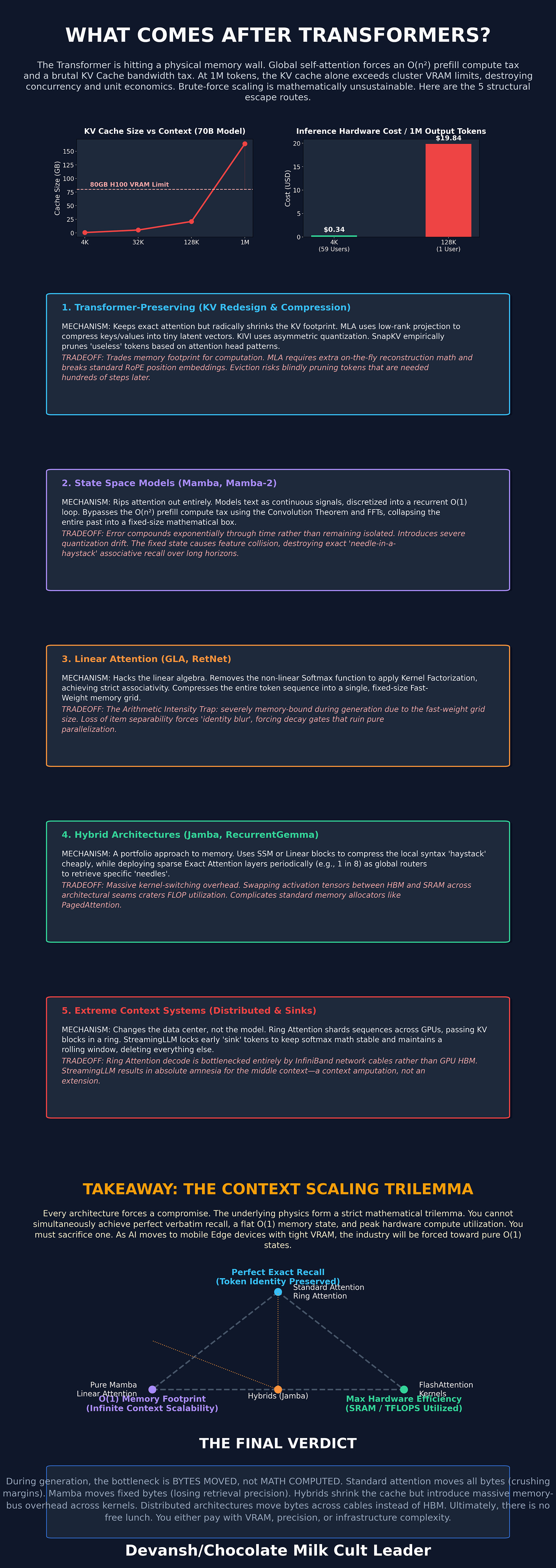
Transformers are running into a hard deployment wall because long-context inference gets expensive in two different ways: prefill suffers from quadratic compute, and decode suffers from a KV-cache memory problem that crushes batching and concurrency. In practice, decode is often memory-bandwidth bound, not compute-bound; the GPU is spending its life hauling cached tokens around instead of thinking. That is why long context wrecks margins. On a 70B model running on an 80GB H100, a 4K context can support roughly 59 concurrent users, but at 128K context that drops to about 1 user. Raw hardware cost jumps from about $0.34 per million output tokens at 4K to roughly $19.84 per million output tokens at 128K. Same GPU; same model; just a much bigger context window. Congratulations, your SaaS now has the unit economics of a hostage situation.
The article then walks through the main escape routes. The first is KV-cache compression: keep attention, but shrink the memory bill with tricks like MLA, KV quantization, pruning, and paged memory. This is the most practical near-term fix because reducing bytes moved directly helps decode. DeepSeek-style MLA, for example, can slash KV size enough that the same 70B at 128K goes from about 1 user per H100 to around 27, and hardware cost falls from about $19.84/M tokens to about $0.73/M. The second path is replacing attention entirely with recurrent or linear-time architectures like Mamba and Linear Attention. These remove KV growth altogether and can make memory stop being the main constraint, but they usually lose sharp token-level retrieval, especially on long contexts where exact recall matters.
The third path is hybrids, which are probably the current engineering sweet spot: use a few attention layers for exact retrieval and cheaper recurrent/compressed layers everywhere else. This pushes the memory wall back without fully sacrificing recall. In the article’s pricing, a Jamba-style hybrid cuts the 70B 128K case down to roughly 14 users per H100 and around $1.42/M tokens in raw hardware cost. Better than vanilla attention; worse than aggressive KV compression; much more realistic than pretending pure recurrent systems have no tradeoffs. The fourth path is distributed exact attention like Ring Attention and Context Parallelism, where you keep full attention but shard the sequence across GPUs. That preserves quality and enables million-token contexts, but it shifts the bottleneck to network bandwidth, especially during decode. Great if you care about capability more than cost; not great if you enjoy money.
The article’s real point is that every post-Transformer design is making the same trade: what are you willing to sacrifice to stop moving so many bytes? Standard attention preserves perfect recall but destroys concurrency and margins at long context. Compression methods save memory but add complexity or quality risk. Recurrent and linear models fix memory growth but lose exact retrieval. Hybrids are the best compromise today. Distributed attention keeps quality, but the bill follows you into the network rack.
This is a long article. If you are very busy, your best bet is to go to the Substack link, and use their navigation system to go the sections that are most interesting to you:
Section 0 — The baseline math: what the quadratic tax actually is (two distinct failures, not one), the KV cache formula, and the hardware roofline that dictates why decode is universally memory-bound.
Section 1 — Keeping the Transformer but shrinking the bill: MLA low-rank compression, token eviction (SnapKV), KV quantization (KIVI), and paged memory (vLLM). Four orthogonal levers you can stack.
Section 2 — Mamba and State Space Models: the control-theory approach to killing the KV cache entirely, the FFT cheat code, why selectivity broke the convolution math, and the quantization error compounding problem that keeps Mamba out of production.
Section 3 — Linear Attention: the algebraic parentheses trick, the 200x concurrency math, and why it always looks clean on benchmarks but never ships at the frontier (feature collision destroys exact retrieval).
Section 4 — Hybrid Transformers (Jamba, RecurrentGemma): the portfolio allocation approach, the residual stream rescue mechanism, the 87% KV cache reduction — and the three friction points (kernel switching overhead, serving stack rewrites, the wall doesn’t disappear, it rotates).
Section 5 — Distributed exact attention (Ring Attention) and StreamingLLM: brute-forcing perfect recall across GPUs vs. amputating the middle and keeping the patient alive.
Section 6 — The full deployment stress-test: KV sizes, concurrency ceilings, and $/M output tokens for 1B, 3B, and 70B models across 4K to 1M context on H100s. Then every escape route re-priced against the worst-case scenario.
I put a lot of work into writing this newsletter. To do so, I rely on you for support. If a few more people choose to become paid subscribers, the Chocolate Milk Cult can continue to provide high-quality and accessible education and opportunities to anyone who needs it. If you think this mission is worth contributing to, please consider a premium subscription. You can do so for less than the cost of a Netflix Subscription (pay what you want here).

I provide various consulting and advisory services. If you‘d like to explore how we can work together, reach out to me through any of my socials over here or reply to this email.
Section 0: Required Background on Costs of AI
Before we analyze how to escape the quadratic tax, we need to define exactly what the tax is, how it is collected, and the physical limits of the hardware paying it.
We’re going to throw a lot of numbers and claims here. If you want to understand where they come from, make sure you read our primer: “The Real Cost of Running AI”, where we derived the costs of running AI from scratch.
What “Breaking the Quadratic Tax” Actually Means
The phrase “quadratic tax” gets thrown around casually to describe why long-context AI is hard. But it is not a single bottleneck. It is two distinct failures occurring in two different phases of inference:
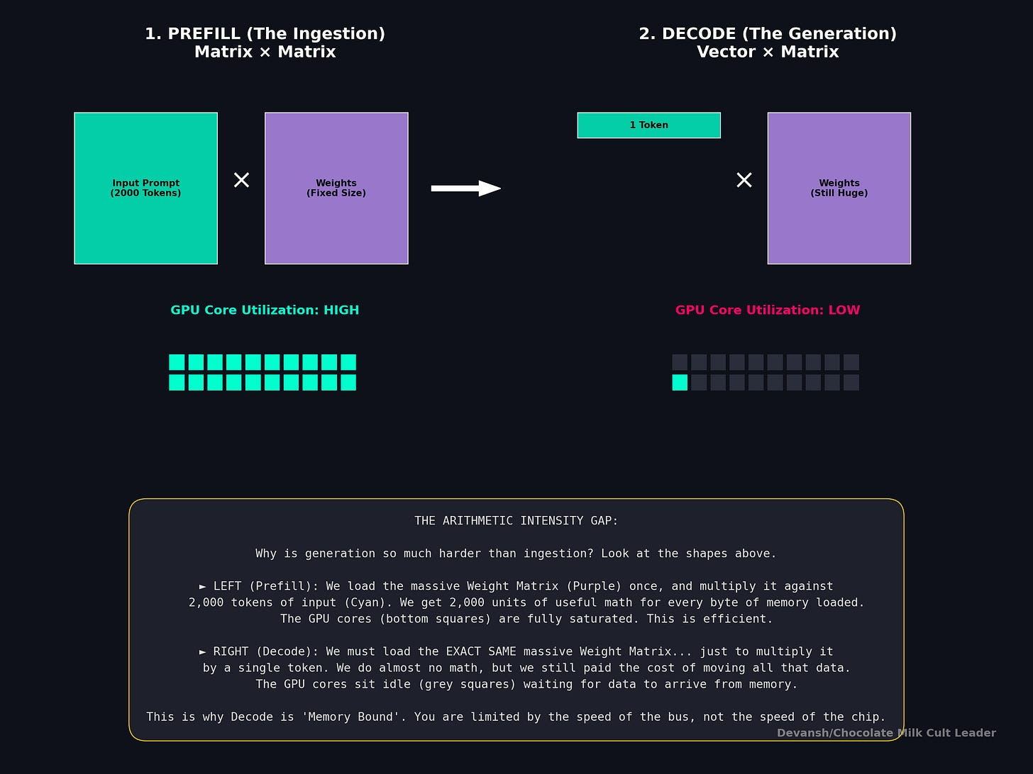
The Prefill Compute Tax: When you hand a prompt to a Transformer, global self-attention forces every token to look at every other token. This creates an irreducible O(n²) computational cost. If you double the prompt length, the math operations quadruple.
The Decode Bandwidth Tax: Once the prompt is processed, the model generates new tokens one by one. To avoid recomputing the entire past, the model caches the Key and Value (KV) vectors for every token. But here is the catch: to generate token n+1, the GPU must read the entire KV cache for tokens 1 through n from High Bandwidth Memory (HBM) into the chip’s processing cores.
At a batch size of 1 (interactive latency), generation is almost entirely memory-bandwidth bound. You are not limited by how fast your GPU can multiply numbers. You are limited by how fast it can physically haul the KV cache across the silicon wire.
This is where we hit a huge misunderstanding around the current ecosystem.
FlashAttention and its successors (like FlashAttention-3) are brilliant I/O-aware algorithms. They greatly reduce memory writes by tiling calculations intelligently on-chip. But they do not change the underlying operation count, and they do not stop the KV cache from growing.
If all tokens attend globally, the cache grows. When the cache grows, it eats the memory you need for batching. When you cannot batch requests, your economics collapse. This is a core mathematical reality that our FA doesn’t help with.
The Mathematical Baseline
To evaluate the escape routes objectively, we need a shared specification. We will use the standard Transformer math.
Here are the terms that dictate the cost of serving:
n: context length (tokens)
d: model width
L: total layers
L_attn: attention layers (some hybrid models use fewer)
h: number of query heads
g: number of KV heads (like in Grouped Query Attention)
d_k: per-head key dimension (often d divided by h)
B_kv: bytes per KV element (2 bytes for FP16, 1 byte for INT8)
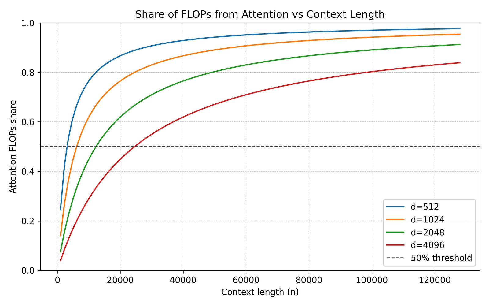
The compute required for a standard Transformer layer (dense attention plus dense MLP) roughly scales as: 24nd² + 4n²d.
That 4n²d part is the global all-pairs term. That is the prefill tax.
But the true dictator of scale is the total size of the KV cache at length n. It is calculated by multiplying: 2 * L_attn * g * d_k * n * B_kv.
This creates a brutal, non-negotiable reality. For every single token you add to the sequence, you pay a fixed bytes-per-new-token tax. If a new architecture does not shrink the number of KV heads (g), the dimension size (d_k), the byte size (B_kv), or eliminate the context length (n) entirely, it has not solved the memory wall.
The Hardware Roofline: Understanding Where Things Break
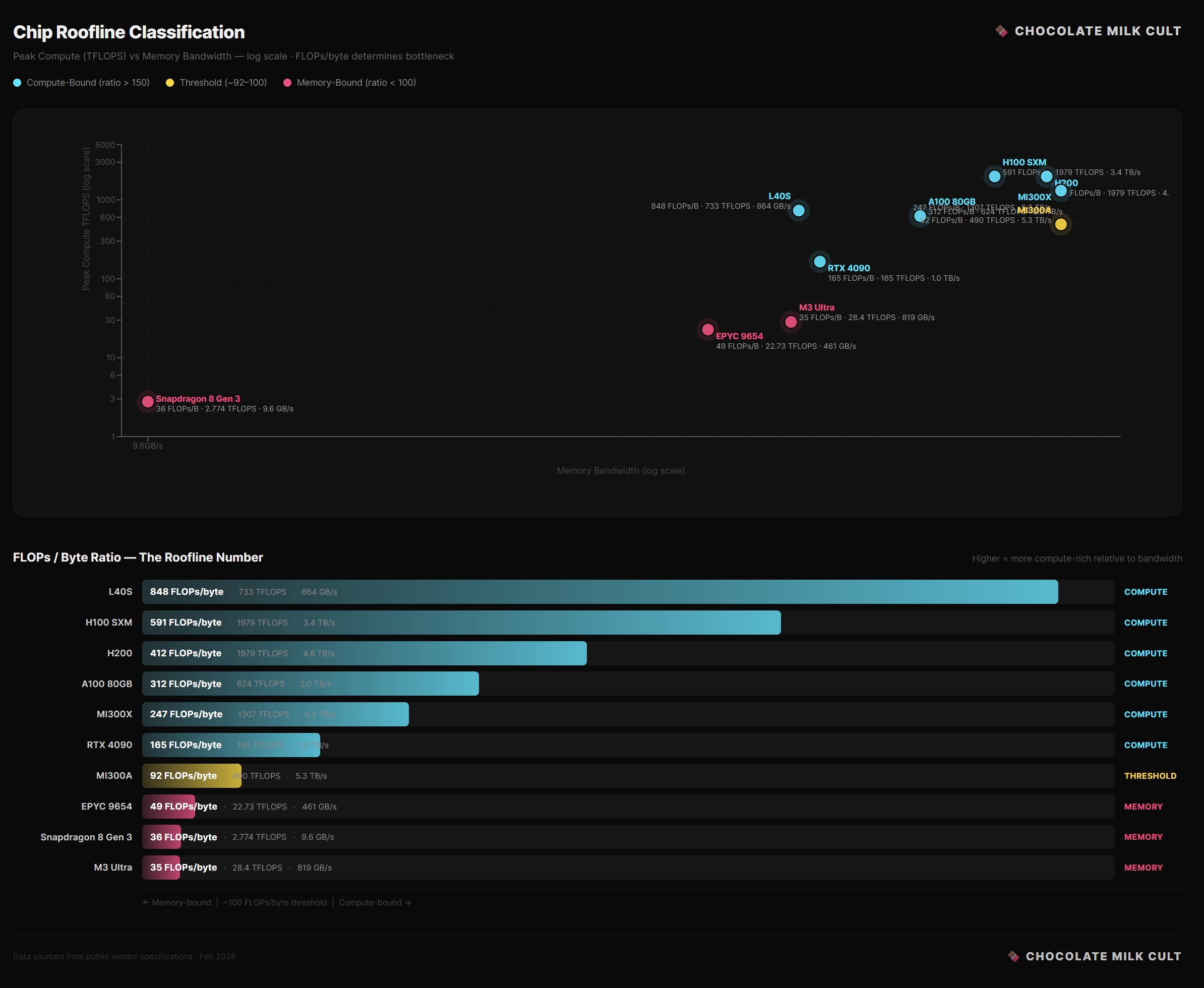
To understand why decode is so painful, we have to look at the hardware’s “roofline” limit. A GPU’s performance is capped by either its peak compute (TFLOPS) or its memory bandwidth (TB/s).
The deciding metric is Arithmetic Intensity: the ratio of math operations performed to bytes loaded from memory (FLOPs divided by Bytes).
Consider the official specs of an NVIDIA H100:
Memory Bandwidth: 3.35 TB/s
FP16 Compute: 1,979 TFLOPS
To hit maximum compute efficiency, the H100 requires an Arithmetic Intensity of roughly 591 FLOPs per byte (1,979 divided by 3.35). If your algorithm does fewer than 591 math operations for every byte it pulls from memory, the processing cores will sit idle, waiting for data.
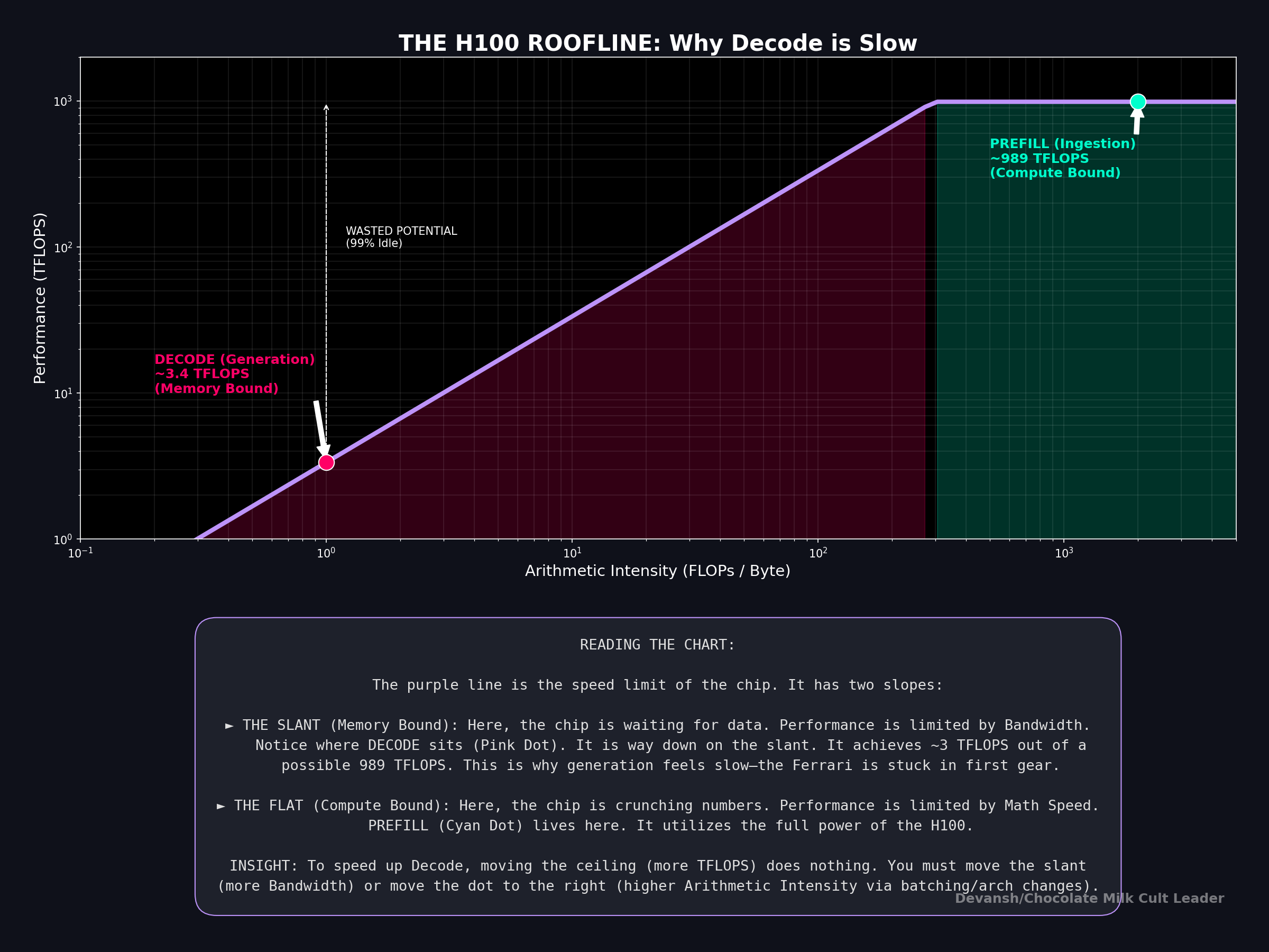
In the decode phase, the model loads the entire massive KV cache just to perform a tiny matrix-vector multiplication for a single token. The Arithmetic Intensity is practically zero.
This is why decode is universally memory-bound. GPUs have evolved to possess massive compute relative to their bandwidth. An architecture that saves FLOPs but moves the same number of bytes is useless for decode. To speed up generation, you must move fewer bytes.
Experimental Constraints
Theoretical elegance is nice, but deployment is a physical game of fit. Throughout this analysis, we will stress-test these theoretical escape routes against realistic conditions.
We will treat quantization as a baseline lever, separated into two buckets:
Weight Quantization (INT8 or INT4): Shrinks the static footprint of the model, leaving more room for the KV cache.
KV Quantization (INT8 down to 2-bit): Directly attacks the per-token memory tax. Extremely impactful at long context, though it risks degrading recall.
Our evaluation constraints:
Target Hardware: NVIDIA H100 80GB and A100 80GB.
Memory Budget: 80GB total, minus a strict 6GB overhead for runtime, allocators, and activations.
Representative Models: 1B, 3B, and 70B parameter proxies.
Context Windows: 4K, 32K, 128K, and the extreme 1M-token boundary.
What this article will be
Putting all this together, we first understand the following:
Faster kernels buy you runway — they don’t lift you off.
Optimizing compute without solving memory simply delays hitting the wall — it doesn’t remove it.
Eventually, serving long-context inference reliably and cheaply requires deeper structural innovation, not incremental kernel tweaks.
This sets up the critical question this article tackles: How do we fundamentally break or sidestep the quadratic reality?
Next, we’ll cover exactly how researchers are answering this challenge.
Section 1: How to Keep the Transformer but Shrink the Memory Bill (KV Cache Compression)
The attention mechanism in a standard Transformer is incredibly good at what it does: fetching highly specific information from anywhere in the prompt. The problem isn’t the attention operation itself; the problem is the storage bill it racks up.
Because of this, the first and most “production-friendly” family of escape routes shares a common philosophy: Do not replace attention. Just change what gets cached, how it is stored, or which parts are retained.
After all, sometimes even when you know the foundation is toxic, and your latency issues will never truly be resolved, the voices in your head remind you that taking a ‘leap of faith’ into a completely new architecture usually just ends with you breaking production on a Friday. In such cases, it’s best to listen to the voices. They know you aren’t a 10x pioneer; you’re just an idiot with a GitHub account, a Claude Code subagent circlejerk, and a rapidly depleting runway. So you stay. You don’t fix the rot; you find ways to deal with it.
If we look back at our KV cache formula (Total Cache = 2 * L_attn * g * d_k * n * B_kv), we can partition the redesign strategies into four orthogonal levers. You can stack these levers to get massive efficiency gains without completely throwing out the Transformer architecture.
1. Shrinking the Hidden Dimension: How Low-Rank Compression Saves Memory. Examples: DeepSeek-V2 (MLA)
Instead of storing massive Key and Value tensors for every token, what if we just store a highly compressed “summary” vector?
This is the exact mechanism behind DeepSeek-V2’s Multi-head Latent Attention (MLA). In standard attention, you cache the Keys and Values. In MLA, you project the token’s information down into a much smaller latent vector. During the decode phase, the GPU only appends this tiny vector to the cache. When it needs to calculate attention, it rapidly “up-projects” or reconstructs the Keys and Values on the fly.
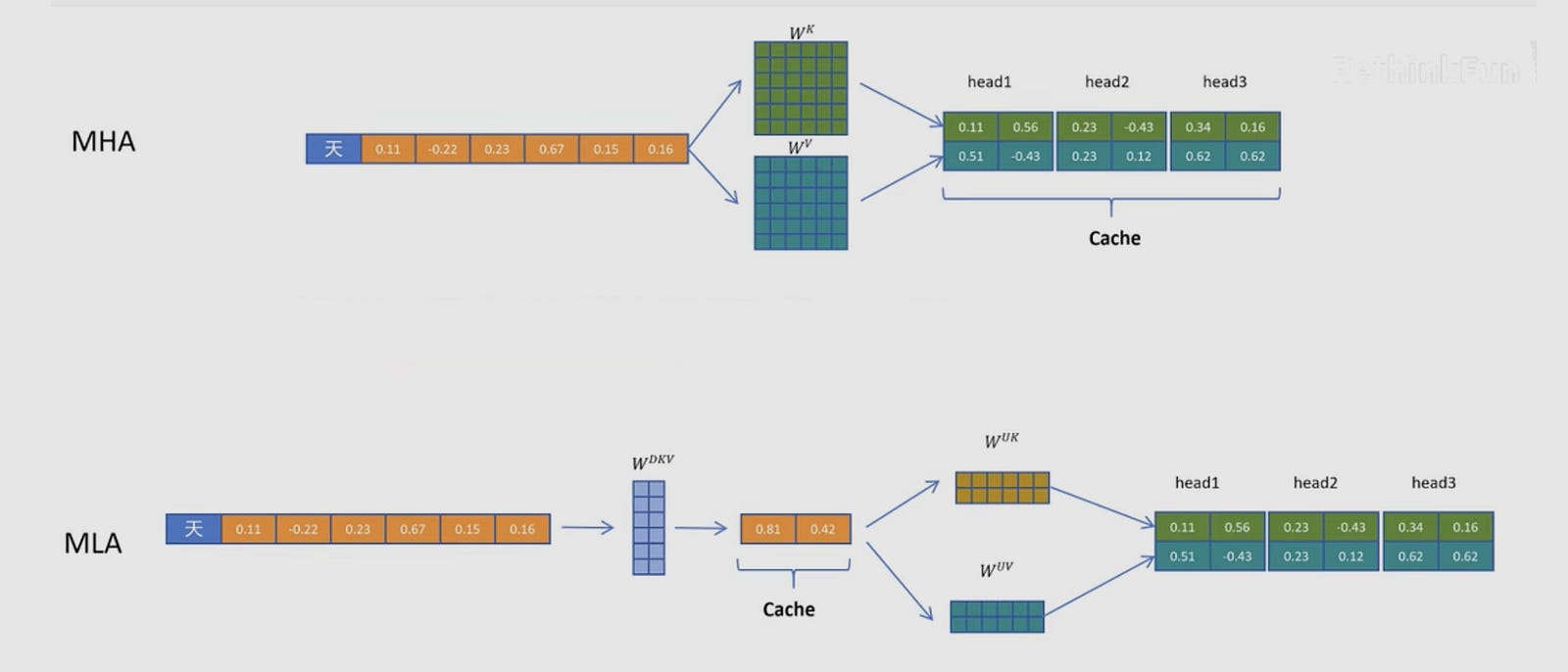
By replacing the large 2 * g * d_k term with a much smaller compressed dimension d_c, DeepSeek reported a staggering 93.3% reduction in KV cache size — “Compared with DeepSeek 67B, DeepSeek-V2 achieves significantly stronger performance, and meanwhile saves 42.5% of training costs, reduces the KV cache by 93.3%, and boosts the maximum generation throughput to 5.76 times.”
Unfortunately, this is not a free lunch. You are trading memory for compute. Reconstructing the keys and values requires an extra matrix multiplication. Furthermore, low-rank compression breaks traditional position embeddings like RoPE (Rotary Position Embedding). Applying RoPE to compressed keys increases their mathematical variance, degrading accuracy unless you implement careful “decoupled” RoPE strategies.
2. Evicting Useless Tokens: How Pruning the Context Saves Memory
Examples: SnapKV, H2O, Expected Attention
If you have a 100K token prompt, do you really need to remember the exact wording of a generic conjunction in paragraph 4? Probably not. Token eviction treats the KV cache as a dynamic optimization problem: out of all candidate tokens, we only want to keep a small subset of size m that minimizes the error in the final output.
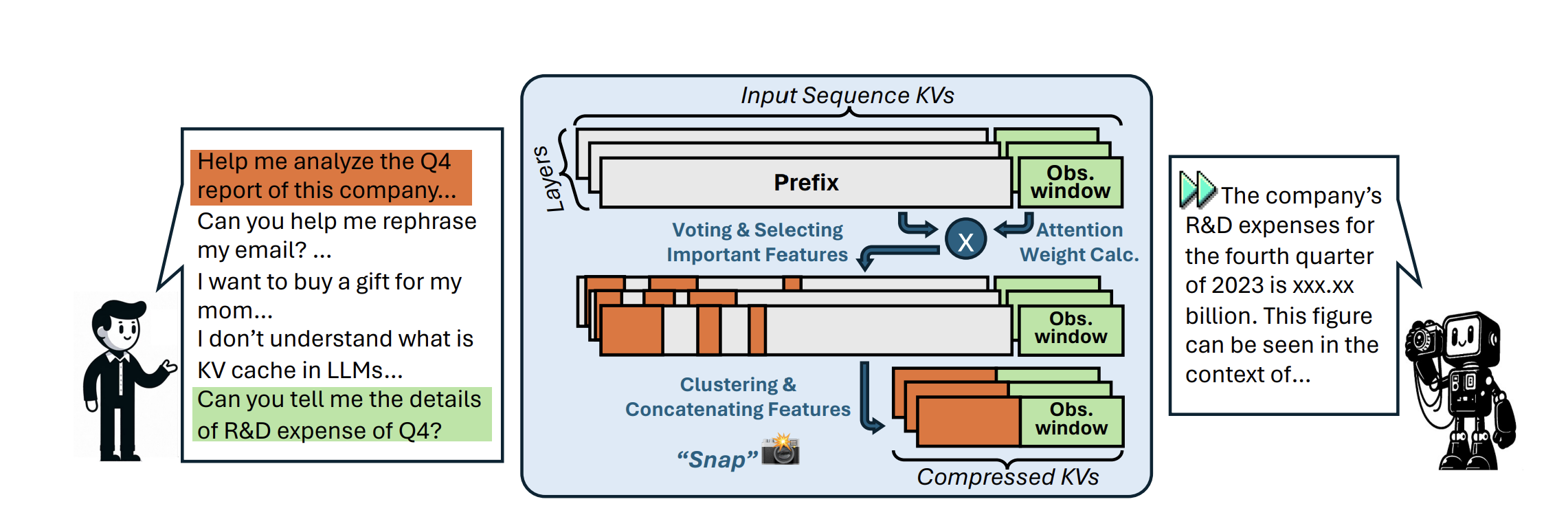
As you might guess, Eviction is incredibly difficult to do perfectly. Why? Because you don’t know what the user is going to ask in the future. You might prune a token that seems irrelevant during the prefill phase, only to realize you needed it 500 tokens into the generation phase. Furthermore, modern fast-attention kernels (like FlashAttention) don’t actually materialize the full attention matrix in memory, making it structurally difficult to see which tokens were historically “important” without adding expensive, custom operations.
3. Using Fewer Bits: How KV Quantization Saves Memory
Examples: KIVI
If you can’t reduce the number of tokens or the size of the vectors, just use fewer bits to represent them. Standard models use FP16 (2 bytes per number). We can quantize this down to INT8 (1 byte) or even 2-bit formats.
The breakthrough in recent papers like KIVI is the realization that the Key cache and the Value cache behave differently. KIVI found that the Key cache has extreme outliers across specific channels, while the Value cache varies mostly token-by-token. By applying asymmetric quantization (quantizing Keys per-channel, and Values per-token), KIVI had some jaw-dropping numbers: “With hardware-friendly implementation, KIVI can enable Llama, Falcon, and Mistral models to maintain almost the same quality while using 2.6× less peak memory (including model weight). This reduction in memory usage enables up to 4× larger batch size, bringing 2.35× ∼ 3.47× throughput on real LLM inference workload”
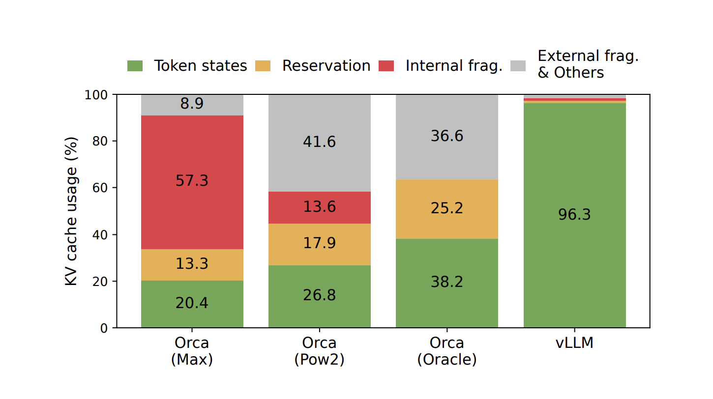
4. Eliminating Waste: How Paged Memory Management Increases Concurrency. Examples: PagedAttention (vLLM)
Sometimes the problem isn’t the math; it’s the memory allocator. Historically, serving engines allocated contiguous chunks of memory for the maximum possible sequence length of a request. If a request ended early, that memory sat empty, leading to massive fragmentation waste.
PagedAttention brought the concept of operating system virtual memory to LLMs. It stores KV blocks in non-contiguous, fixed-size pages. This virtually eliminates fragmentation and allows different requests to share the same cached prefixes (like system prompts), drastically increasing the number of users you can serve concurrently on the same GPU.
This is likely my favorite technique since it’s basically the digital slumlord model of memory management: pack the contexts into non-contiguous studio apartments, charge premium API rates, and just pray your users don’t all trigger a 32K context generation at the exact same time. And as they say, dress for the job you want.
Summary: The Hardware Tradeoffs of KV Compression
How do these methods map to our hardware reality?
They directly attack the “Bytes” side of the Arithmetic Intensity equation. Because decoding is so aggressively memory-bound (especially at low batch sizes), taking on a little bit of extra math (like MLA’s reconstruction steps or eviction’s scoring logic) to drastically reduce the amount of data pulled from HBM is almost always a winning trade.
But as context windows stretch toward 1 million tokens, even a compressed cache eventually hits a wall. To truly eliminate the growth of n (the context length), we have to look at architectures that rip the attention mechanism out entirely.
And this is where things get a bit funky.
Section 2: Attention-Replacing Escape Routes (Deleting the Context Length)
Compressing the KV cache is a great short-term survival strategy. But fundamentally, you are still playing a losing game. As long as your memory grows with the context length (n), you will eventually hit a wall where your batch size drops to zero and your economics collapse.
To truly fix the quadratic tax, we have to look at architectures that rip standard attention out of the model entirely.
The goal of these “attention-replacing” escape routes is simple: achieve O(1) memory during generation. This means whether you are on token 100 or token 1,000,000, the amount of memory required to store the past stays exactly the same.
To do this, you have to stop storing a list of every token you’ve ever seen, and start compressing the entire past into a fixed-size mathematical box.
Let’s unpack the most prominent attempt to do this: State Space Models (SSMs) and Mamba.
Why Continuous Time? The Intuition Behind State Space Models
If we want to compress the past into a box, we need a mathematical way to describe how that box should change when new information hits it.
Think about how you track the temperature of a room. You don’t memorize every single temperature reading from the last 10 years (which is what a Transformer does with the KV cache). You just have a current temperature (the state), and when the AC turns on (the input), the temperature changes.

Control theory spent a century figuring out how to track changing physical systems like this — whether it’s an airplane on radar, thermostat, or the runway of an AI wrapper where the API costs are higher than actual revenue. Early SSM papers (like S4) realized that if we treat a sequence of tokens not as a list of discrete words, but as a continuous flowing signal, we can borrow all this proven math to model change with differential equations.
To figure out how, let’s look at the exact behavior we want to enforce:
We have a box that holds our compressed memory: let’s call it x(t).
We have a new piece of information arriving: let’s call it u(t).
We need to know how the box changes over time: dx/dt.
To calculate that change, we need two forces pulling on the box.
The Decay Force: How much of the old memory should survive, and how much should fade away? We multiply the current state x(t) by a learned matrix A.
The Input Force: How much should this brand-new token alter the state? We multiply the new input u(t) by a learned matrix B.
Put them together, and you get the core engine of an SSM:
dx/dt = A * x(t) + B * u(t)
The matrix A is the absolute dictator of this system. It controls the memory timescales. If the numbers in A are set correctly, the system is stable — it slowly forgets useless old information while safely absorbing new inputs. Once the state is updated, we just multiply it by another matrix to pull our final answer out of the box.
Discretization: Turning the Ramp into Stairs
This continuous math is beautiful for tracking smooth audio waves. But language isn’t a smooth wave. It arrives in discrete, choppy chunks: Word 1, Word 2, Word 3.
To reconcile this, we have to “discretize” the math. We introduce a step size (Delta) to convert our continuous matrices A and B into discrete step-by-step matrices, A_bar and B_bar.
Now, the math becomes a simple recurrent loop: New State = (A_bar * Old State) + (B_bar * New Token)
Look at the economic consequences of this equation. Because we only need the Old State to compute the New State, the moment the math is done, we completely throw the New Token away. We do not cache its Key. We do not cache its Value. The KV cache drops to exactly zero.
The Convolutional Cheat Code: The Exact Math of Bypassing O(n²)
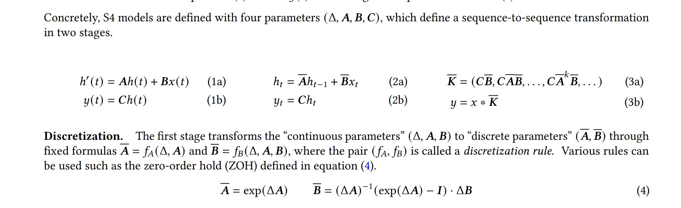
To understand how State Space Models (SSMs) eliminate the prefill tax, we have to look at the exact algebra of the recurrent loop.
Let’s assume our starting state is zero (x_0 = 0). Here is the discrete update rule for the hidden state (x) and the output (y) at each step:
x_t = (A_bar * x_{t-1}) + (B_bar * u_t)
y_t = C * x_t
If we unroll this step-by-step for the first three tokens, substituting the previous state into the current one, the algebra looks like this:
x_1 = B_bar * u_1
x_2 = (A_bar * B_bar * u_1) + (B_bar * u_2)
x_3 = (A_bar² * B_bar * u_1) + (A_bar * B_bar * u_2) + (B_bar * u_3)
Notice what is happening to the input tokens (u). The older the token, the more times it gets multiplied by the decay matrix A_bar.
Because we want the final output y, we multiply these states by the output matrix C. This allows us to define a single, massive Convolution Kernel (K). This kernel represents the exact mathematical multiplier for how much a token from k steps ago affects the output today:
K = [C * B_bar, C * A_bar * B_bar, C * A_bar² * B_bar, …, C * A_bar^(n-1) * B_bar]
Because A_bar, B_bar, and C are fixed matrices (Time-Invariant), we can pre-compute this entire list of multipliers before the model even looks at the prompt.
Once we have K, the output vector y for the entire prompt is simply the mathematical convolution of the input sequence u and the kernel K:
y = K * u
The O(n²) Problem with Native Convolution
We have eliminated the step-by-step recurrent loop, but we have not solved our compute problem yet.
The standard mathematical definition of discrete convolution requires computing the sum of the products for every overlapping point. To compute the output at token 100, you multiply the first 100 elements of u by the first 100 elements of K (in reverse). To do this for every token from 1 to n, the number of multiplications scales as 1 + 2 + 3 … + n.
That arithmetic progression resolves to (n² + n) / 2.
And just like that, we are right back where we started: an O(n²) prefill tax. You really can’t get anything to work, huh? Now is a good time to seriously consider that the universe hates you and wants you to pay Daddy Jensen more money.
Don’t give up yet, though. Lucky for you, we can ass pull a mathematical loophole that makes SSMs viable: the Convolution Theorem.
The Convolution Theorem and the FFT
The theorem proves a fundamental property of linear algebra: a convolution in the time domain is mathematically identical to element-wise multiplication in the frequency domain.
The equation is: FFT(y) = FFT(K) ⊙ FFT(u)
(Where FFT is the Fast Fourier Transform, and ⊙ is element-wise multiplication).
Here is the exact step-by-step operation the GPU performs, and the cost of each step:
FFT of the Input (u): The GPU converts the sequence of tokens into the frequency domain. The standard Discrete Fourier Transform requires an n × n matrix multiplication (O(n²)). But the Fast Fourier Transform algorithm exploits the recursive symmetry of sine and cosine waves to divide-and-conquer the matrix, cutting the exact compute cost down to O(n log n).
FFT of the Kernel (K): We do the same thing to our pre-computed kernel. Cost: O(n log n).
Element-wise Multiplication: We take the two transformed lists and multiply them together, one-to-one. No massive matrix multiplies, just array_A[i] * array_B[i]. Cost: exactly O(n).
Inverse FFT: We take the resulting frequencies and run the Inverse FFT to transform them back into the final token outputs y. Cost: O(n log n).
By taking this mathematical detour, we have replaced an O(n²) operation with three O(n log n) operations and one O(n) operation.
At a context length of 4K, the difference is negligible. But at a context length of 1 million tokens, n² is 1 trillion operations. n log n is roughly 20 million operations.
By applying the Convolution Theorem, we mathematically annihilate the prefill compute tax.
The Mamba Breakthrough: Why “Selectivity” Broke the Math
If this math is so flawless, why did these models underperform Transformers on text?
Look at the definition of our kernel K:
K = [C * B_bar, C * A_bar * B_bar, C * A_bar² * B_bar…]
This kernel assumes that A_bar and B_bar are static numbers. They treat every single position in the sequence exactly the same. But language requires content-adaptive memory. A model needs to forget a filler word like “um” instantly, but lock a critical noun into memory for 50,000 steps.
Mamba fixed this by introducing Selectivity. It makes the matrices A_bar and B_bar input-dependent. The model learns a gating mechanism that changes the values of A_bar and B_bar for every single token (which makes intuitive sense, different tokens create different pressures on what needs to be retained).
But this creates another problem.
If A_bar changes at every step, you can no longer pull it out and create a single, static Kernel K.
K no longer exists. y = K * u is mathematically impossible. The Convolution Theorem breaks. You are forced back into computing the sequence step-by-step.
This is exactly why Mamba’s engineers had to invent the complex “Associative Scan” kernels. Let’s study them next.
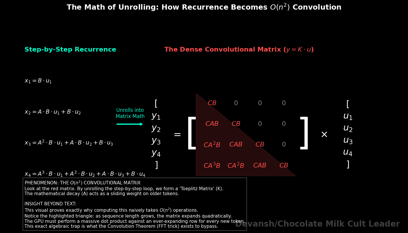
The Engineering Reality: The Math of the Associative Scan
We lost our little O(n log n) FFT cheat code. We are forced back into computing the sequence step-by-step because Mamba’s matrices A and B now change at every time step t (which we will now write as A_t and B_t).
The recurrence is:
x_t = (A_t * x_{t-1}) + (B_t * u_t)
If you code this as a standard for loop on a GPU, performance collapses. The GPU has thousands of cores; a sequential loop forces one core to work while the rest sit idle.
To parallelize this, the Mamba authors relied on a computer science algorithm called a Parallel Prefix Sum (or Associative Scan).
To make a scan work, you must define a mathematical operation that is strictly associative — meaning (X ⊗ Y) ⊗ Z must equal X ⊗ (Y ⊗ Z). If it is associative, you can group the sequence into chunks, calculate the chunks on different GPU cores at the exact same time, and combine the results in a tree structure.
But our update rule isn’t just simple addition. It’s a matrix multiplication and an addition. How do we make that associative?
We define a new operator (let’s call it ⊗) that operates on a pair of values: the decay matrix A, and the input projection B * u.
If we have two adjacent time steps, i and j, the operator is defined as:
(A_i, B_i * u_i) ⊗ (A_j, B_j * u_j) = (A_j * A_i, A_j * B_i * u_i + B_j * u_j)
Because this specific combination of multiplying the old state and adding the new input is mathematically associative, we can chunk the prompt. Core 1 computes the exact tuple for tokens 1–10. Core 2 computes tokens 11–20. They do this in parallel, then merge their tuples up the tree.
But our issues don’t end here.
And since the creators of Mamba have not agreed to my demands to a yacht party with crystals of chocolate milk that I can snort off hookers, let’s end this section with a discussion of the biggest issues with Mamba currently.
Why Mamba isn’t the Status Quo (Yet)
In standard Attention, you load two massive matrices (Q and K) into the GPU’s ultra-fast Tensor Cores and multiply them. It requires an astronomical amount of math, but it has incredibly high Arithmetic Intensity. The cores crunch numbers without having to constantly wait on memory.
Look at our custom scan operator ⊗. We are doing a few small matrix-vector multiplications, but to execute the tree structure, the GPU threads have to constantly read and write these (A, B*u) intermediate tuples to the chip’s SRAM.
The eagle-eyed amongst you would have noticed are doing very little actual math per byte of data moved. You have successfully parallelized the O(n) computation, but you have created an algorithm that is ruthlessly memory-bound. Writing a custom CUDA kernel that handles this memory traffic without stalling the GPU is one of the hardest software engineering problems in AI right now. Even with brilliant implementation, Mamba’s core layers struggle to hit the peak hardware utilization numbers that standard Transformer matrix multiplication achieves effortlessly.
Along with this, there is ANOTHER problem that Yamchas many deployments of Mamba.
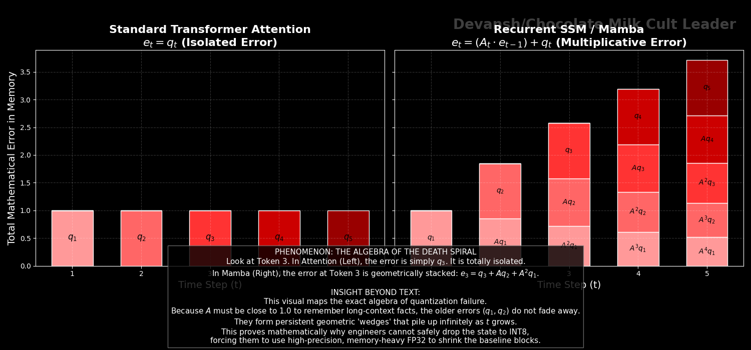
In a Transformer, dropping your KV cache to INT8 or INT4 quantization is relatively safe. You are just reading a slightly blurry memory. If token 5’s Key vector is slightly off, it only affects token 5. The error is isolated.
Let’s look at the algebra of what happens when you quantize a recurrent model.
When you quantize the state update, you introduce a small rounding error at every step. Let’s call this error q_t. Our update rule becomes:
x_t = (A_t * x_{t-1}) + (B_t * u_t) + q_t
To see how this error behaves over time, we have to look at the difference between the “perfect” state and our “quantized” state. Let’s unroll the accumulated error e_t over three steps:
e_1 = q_1
e_2 = q_2 + (A_2 * q_1)
e_3 = q_3 + (A_3 * q_2) + (A_3 * A_2 * q_1)
Notice the fundamental difference between this and a Transformer. The quantization noise from token 1 (q_1) doesn’t just sit there. It gets multiplied by A_2. Then it gets multiplied by A_3.
In a nutshell, Recurrent systems don’t just accumulate error; they multiply it through time.
A tiny INT8 rounding mistake at the start of a 100,000-token prompt will compound exponentially until the mathematical state completely blows up and the model starts outputting garbage.
This is why the official Mamba repository explicitly warns that SSMs are highly sensitive to their recurrent dynamics. To prevent this compounding failure, engineers are often forced to store the recurrent state in high-precision FP32 (4 bytes per number).
So you win infinite context (technically, how much of that is useful, especially when it comes to precision heavy tasks that require exact wordings is debatable) and massive concurrency, but you invite a massive kernel engineering and quantization headache.
What happens if we decide that Control Theory is no good? Up next, we will look at how Linear Attention tries to achieve the exact same O(1) memory goal, but it does it entirely through algebra instead of differential equations.
Section 3: Linear Attention and Fast-Weights (Algebraic Factorization)
State Space Models try to kill the context length using differential equations and control theory. But what if you don’t want to learn an entirely new branch of mathematics? What if you just want to take the Transformer we already have, and hack the linear algebra so it stops eating our GPUs?
This is the exact goal of Linear Attention. It attempts to keep the “query-key retrieval” architecture of a standard Transformer, but uses a mathematical loophole to completely bypass the O(n²) prefill tax and the growing KV cache.
To understand how it does this, we have to isolate the exact mathematical operation that chains us to O(n²): the Softmax function.
The Villain: Why Softmax Forbids Associativity
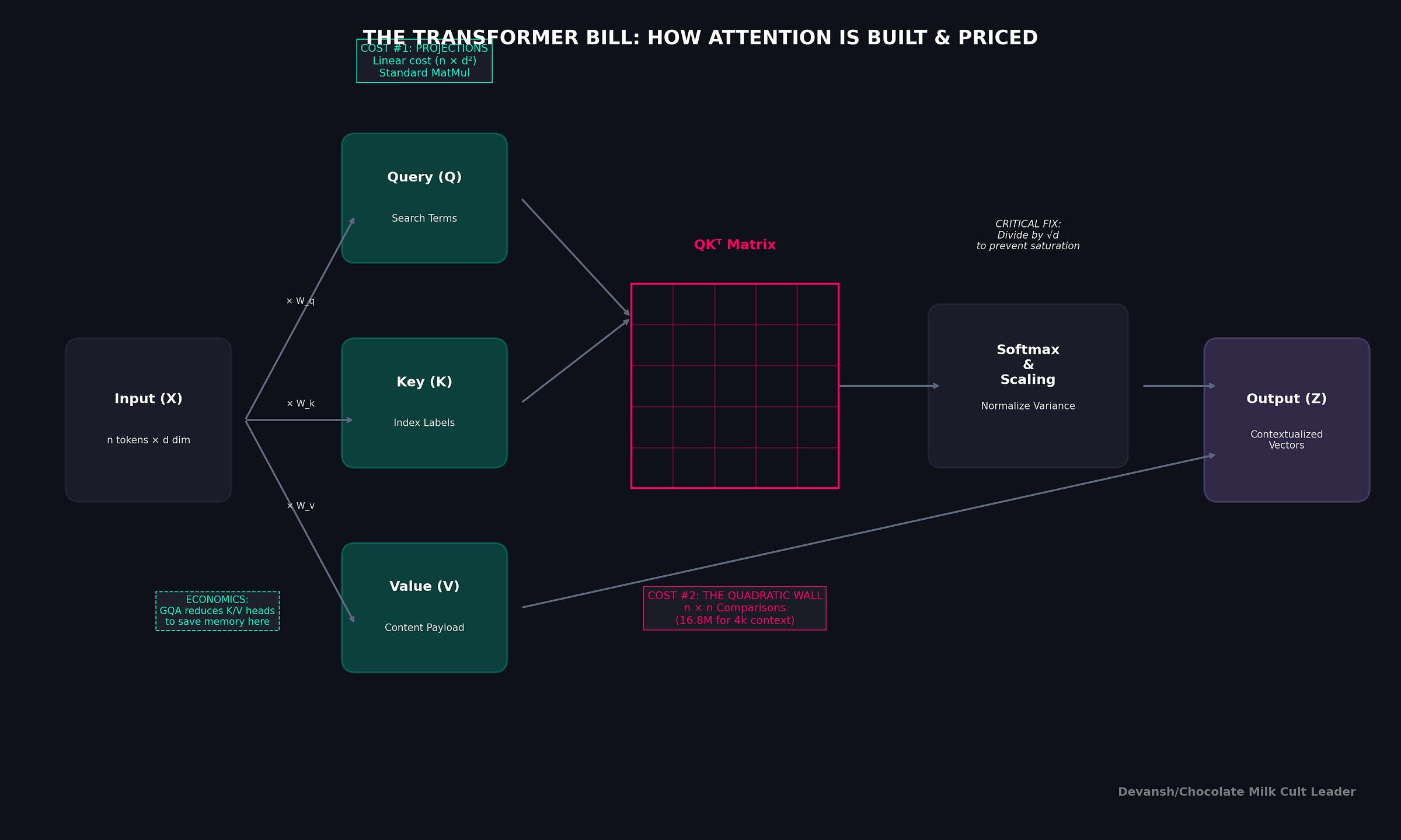
In Part 1, we established the core attention equation: Output = Softmax(Q * K^T) * V.
To figure out how much token A cares about token B, we multiply their Query and Key vectors together to create an n × n matrix of raw scores. We then wrap that matrix in a Softmax function.
Softmax exists for two critical reasons:
Sharp Selective Retrieval: It creates a normalized similarity distribution. It forces the model to pick exactly which past tokens matter, acting as a strict 100% attention budget.
Statistical Stability: Without normalization, if you add up 100,000 raw dot products, the magnitude of the aggregated vector grows proportional to the sequence length. Variance explodes, and the model’s internal activations blow up.
But Softmax comes with a fatal structural cost: it is a non-linear function.
Mathematically, you cannot distribute a matrix multiplication through a non-linear boundary. You cannot regroup the variables. You are algebraically trapped. The GPU must calculate the massive n × n matrix of (Q * K^T) first. You physically cannot change the order of operations, which means you are permanently chained to O(n²).
The Hack: Kernel Factorization
To escape, researchers use a trick called Kernel Factorization.
What if we remove Softmax entirely, and instead apply a non-linear feature map (let’s call it Φ) independently to Q and K before we multiply them? For example, applying a function like ELU(x) + 1 simply forces all the vectors to be positive. (In many linear attention papers like Performer, this is actually used to approximate the original Softmax kernel without computing the n × n matrix).
We change the math from Softmax(Q * K^T) to Φ(Q) * Φ(K)^T.
Because Φ is applied individually to the vectors, the relationship between Q and K is now strictly bilinear. And bilinearity unlocks the greatest cheat code in matrix algebra: Associativity.
Associativity is the rule that says (A * B) * C is the exact same thing as A * (B * C). You can group the multiplications however you want, and you will get the exact same answer.
The Algebraic Escape Route: Moving the Parentheses
Let’s look at the exact matrix dimensions of what happens when we regroup the variables.
Our Query matrix Q has dimensions (n × d).
Our Key matrix K^T has dimensions (d × n).
Our Value matrix V has dimensions (n × d).
The Standard Way (The Quadratic Tax):
We calculate (Q * K^T) first.
An (n × d) matrix times a (d × n) matrix produces a massive (n × n) matrix. This is the global attention map.
We multiply that (n × n) matrix by V (n × d) to get our final output (n × d).
The Linear Attention Way:
We move the parentheses. Instead of (Q * K^T) * V, we calculate Q * (K^T * V).
We calculate (K^T * V) first.
A (d × n) matrix times an (n × d) matrix produces a (d × d) matrix.
We multiply Q (n × d) by that (d × d) matrix to get our final output (n × d).
Look closely at that middle step. We created a (d × d) matrix.
There is no n in that matrix.
By computing K^T * V first, we have compressed the entire sequence of 100,000 tokens into a fixed-size mathematical block. We just created a Fast-Weight Memory. (This concept traces back to Jürgen Schmidhuber (isn’t that funny?) in the early 1990s — the idea of one neural network generating weights for another network on the fly. It failed because 90s hardware couldn’t handle the compute, but modern GPUs can).
During generation (decode), we don’t need to read a massive KV cache anymore. We just maintain this single, fixed-size historical state matrix (let’s call it S_t).
When a new token arrives, the update equation is simple:
S_t = S_{t-1} + (Φ(k_t) * v_t^T)
We take the new token’s Key and Value, multiply them together to create a rank-1 (d × d) grid, and literally add that new grid to our historical state. The moment we add it, we throw the token away. Constant memory. O(1) generation.
The Economics: Pricing the Capacity Unlock
Let’s put actual byte counts on this “fixed” state, because constant memory sounds like a free lunch until you calculate the size of the constant.
Let’s use our 14B model proxy from Part 1: 40 layers, 40 attention heads, and a head dimension (d_k) of 128.
In Linear Attention, you have to store a (d_k × d_v) matrix for every single head.
Size per head: 128 × 128 = 16,384 parameters.
Across 40 heads: 655,360 parameters.
At FP16 (2 bytes per param): ~1.3 MB per layer.
Across all 40 layers: 52.4 MB of total fixed state.
What does 52.4 MB mean for your profit margins?
Let’s look at an 80GB H100. A 14B model at INT4 takes up ~7GB of memory. Framework overhead takes ~6GB. You have roughly 67GB left for users.
At 128K context (Standard Attention): Assuming a highly optimized model using Grouped Query Attention (GQA with exactly 8 KV heads), the KV cache is ~10.4 GB per user. 67GB / 10.4GB = 6 concurrent users.
At 128K context (Linear Attention): The state matrix is 52.4 MB. 67GB / 0.052GB = ~1,288 concurrent users.
From a pure capacity standpoint, that is a 200x revenue multiple on the exact same silicon.
The Hardware Reality: The Arithmetic Intensity Trap
But capacity is only half the battle. We have to look at bandwidth and generation speed.
To generate a single token, the GPU still has to load that 52.4 MB state from High Bandwidth Memory (HBM) into its SRAM cores, update it, and write it back.
Let’s calculate the Arithmetic Intensity (FLOPs per byte) for this operation:
Bytes moved: 52.4 MB.
FLOPs performed: Updating the matrix and calculating the output requires exactly 4 * d_k² operations per head. Across the whole model, that comes out to roughly 105 million FLOPs.
Arithmetic Intensity: 105 MFLOPs / 52.4 MB = 2 FLOPs / byte.
Remember the Roofline model from Part 1? The H100 (using TF32 Tensor Cores) requires roughly 295 FLOPs/byte to be compute-bound. (If you use the FP16 peak marketing numbers, it’s nearly 591 FLOPs/byte).
At 2 FLOPs/byte, Linear Attention is catastrophically memory-bound.
A sharp engineer will immediately object: “Wait, modern kernels like FlashLinearAttention use SRAM tiling and chunking to overlap transfers and keep the state on-chip!”
This is true. Hardware-aware kernels drastically reduce intermediate reads and writes. But you still must load the final 52.4 MB state from HBM for every generation step. Even with perfect tiling, your arithmetic intensity remains orders of magnitude below the roofline limit.
The Regime Analysis: When Do You Actually Win?
Because the fixed state is 52.4 MB, Linear Attention is actually slower and more memory-intensive than a Transformer at short context lengths.
Under 4K tokens: The standard KV cache is smaller than 52 MB. Linear attention loses.
At ~32K tokens: The capacity lines cross. Linear attention breaks even.
At 128K+ tokens: Linear attention becomes a physical necessity for survival.
The Structural Flaw: Feature Collision and Loss of Identity
Even if you deploy in the 128K+ regime, Linear Attention has a physical, mathematical limitation that ruins it for precision-heavy use cases like coding or RAG.
Look back at the update rule: S_t = S_{t-1} + (k * v). We are using additive compression.
A standard Transformer separates every single token. The KV cache perfectly preserves distinct token identities. If you ask it to find a specific needle in a 1-million-token haystack, it can perfectly isolate that exact token’s Key.
Linear attention takes 100,000 distinct token associations and compresses them into a single matrix via additive updates. Over long sequences, these features collide. You lose item separability. The model physically loses the capacity for sharp, exact associative recall because the distinct token identities blur into a single overlapping grid.
The Fix that Breaks Everything: Decay Gates
To stop the state matrix from blurring into useless noise, modern fast-weight variants (like Gated Linear Attention and DeltaNet) introduce a decay gate (γ).
S_t = (γ * S_{t-1}) + (Φ(k_t) * v_t^T)
This forces the model to slowly forget old information. But look at what γ just did to our math. Because γ is a time-dependent multiplier that changes at every step based on the input, the operation is no longer a simple, order-independent sum. It is a time-dependent recurrence.
You just broke pure associativity.
Because the decay at step 100 depends on the decay at step 99, you can no longer process the prefill perfectly in parallel. You are forced into chunkwise recurrent or associative scan algorithms to parallelize training, exactly like RetNet and modern Mamba implementations.
Furthermore, because you are repeatedly multiplying the state by γ, you can accumulate numerical error over long horizons. This makes aggressive low-precision deployment (like INT8) much harder to stabilize without the state drifting.
Linear Attention successfully kills the KV cache, but in the end all must bend the knee to a brutal law of AI economics: you either pay for your context with memory (KV cache), or you pay for it with precision (item separability). There is no free lunch.
Linear Attention variants are very interesting to study in depth since they always have amazing benchmark results on paper. Benchmarks look clean, the math checks out, and there’s never any reason it shouldn’t work. It’s why the Spreadsheet merchants pretending to be AI Influencers/Thought Leaders eat that shit up, and every LA drop is accompanied by a lot of hype about how groundbreaking the whole thing is. And that’s why we don’t see this trickle into innovation at the frontier.
All this being said, I wouldn’t be talking about if LA didn’t have something useful for us to learn. After all, what good is it spend our time on losers that didn’t work out?
Section 4: Hybrids Transformer Networks: Best of Both Worlds ?
In Section 2, we looked at State Space Models (Mamba) which achieve infinite context but suffer from feature collision. In Section 3, we looked at Linear Attention, which unlocks massive batch sizes but loses the ability to do exact, item-separable retrieval.
Both architectures proved the same brutal law of AI economics: you either become a fat fuck and eat that massive KV cache, or you accept brain damage and lose precision. No free lunches here.
But go back and read that law carefully. It says you have to pay. It doesn’t say you have to pay the same way everywhere.
You can choose where in the network you eat each cost. Compress the haystack cheaply in some layers. Retrieve the needle exactly in others. The tradeoff doesn’t have to be global. You do not have to ruin the whole network at once. You can distribute the suffering across depth like a civilized society, the way a portfolio manager allocates risk across asset classes instead of going all-in on one bet.
After all, you are not OpenAI. You do not have a sovereign wealth fund backing your compute cluster. You are a CTO of an AI wrapper whose bad infra decision away from explaining to the board why company lunches now consist of biting the dust, despite your brilliant models and beautiful demos. Best of luck explaining that to the bright-eyed Queens who invested in your little marketing automation startup on the promise that you will rock them.
So, you need to start optimizing things by trying to salvage the best of both worlds. How do we do that?
If we take the portfolio metaphor literally (and we should, because the math maps almost perfectly), the architecture becomes a highly operational trade-off with observable metrics:
The % of Attention layers defines your strict memory budget. Observable metric: KV bytes per token. This dictates your maximum context length at a fixed VRAM limit. Non-negotiable. Hardware doesn’t care about your architecture preferences.
The spacing between Attention layers defines your retrieval latency in depth. Observable metric: needle survival distance — the number of consecutive compressor layers a distinct token identity can pass through before it blurs beyond reliable recovery. Empirically, this appears to sit in the range of 4 to 8 layers for current Mamba-class compressors before needle-in-haystack accuracy starts to degrade sharply, though the exact number is task-dependent. Verbatim string recall dies first. Semantic gist survives longer. Space your attention layers further apart than this survival distance and tasks requiring exact matching — coding, multi-hop RAG, citation retrieval — degrade first, because distinct token identities blur inside the compressed layers before an attention layer can rescue them.
The SSM blocks act as cheap local feature extractors, compressing the “haystack” (the syntax, tone, general narrative).
The Attention blocks act as global routers, scanning the entire sequence to perfectly retrieve the “needle.”
Let’s look at exactly how this is constructed, the math of why it works, and the severe systems engineering friction that prevents it from being a magical silver bullet.
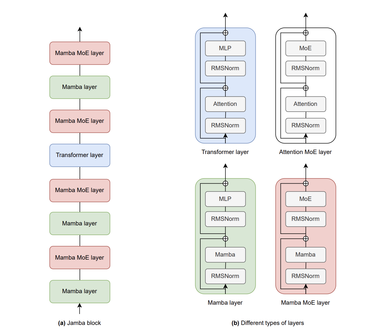
How Do You Wire a Hybrid Transformer Together?
You can’t just throw a sub-quadratic layer and an Attention layer into a blender. You have to route the information.
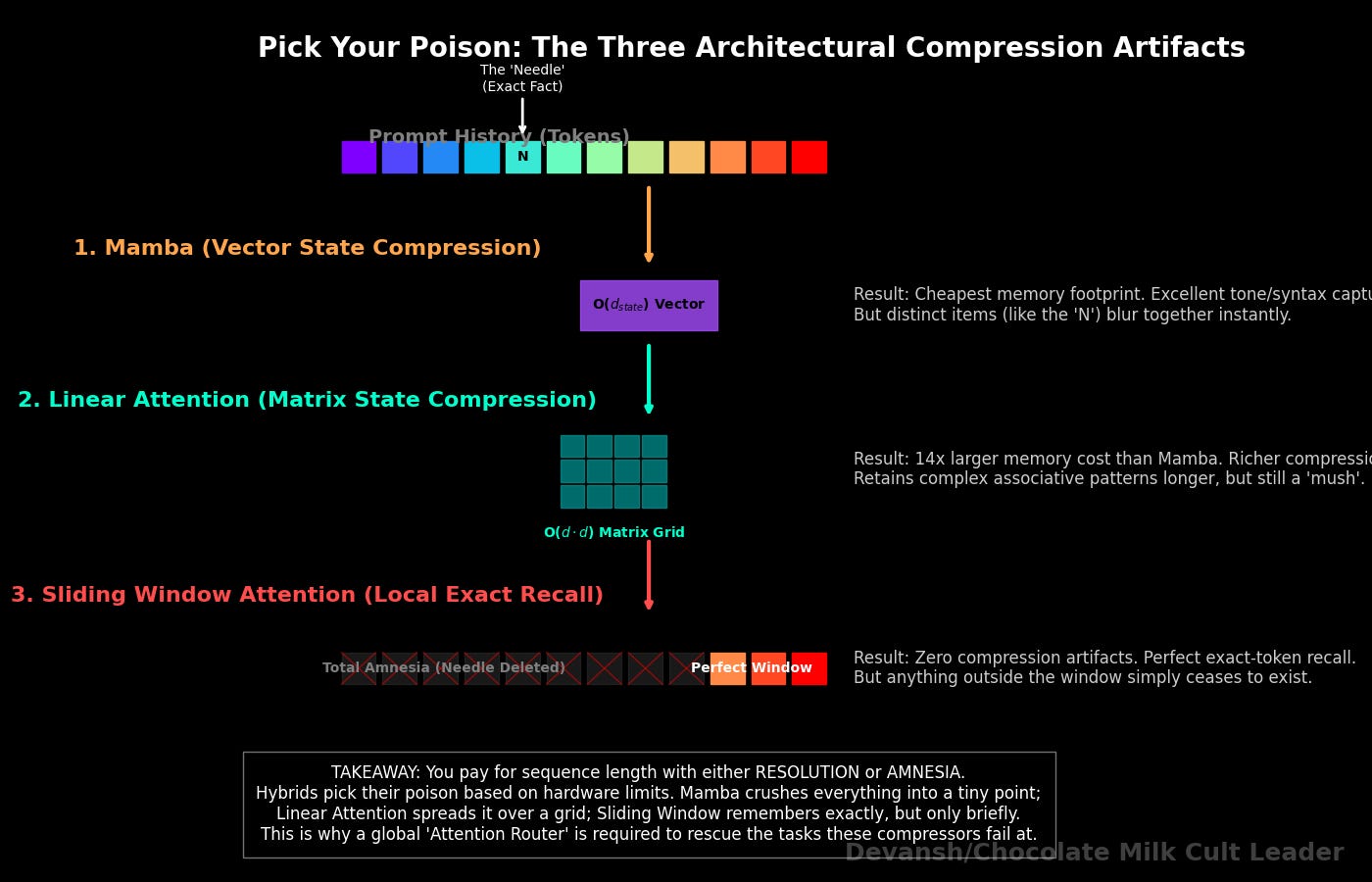
While AI21’s Jamba uses Mamba as its compressor, the industry is experimenting with multiple variants of this portfolio approach. You can swap Mamba out for Linear Attention (GLA/DeltaNet), or even sliding-window local attention. The compressor choice changes the type of compression artifact you get so you can pick your poison based on your hardware and your retrieval requirements.:
Mamba collapses into a fixed recurrent vector of size O(d_model * d_state). What you get: the cheapest possible compression per layer, tiny memory footprint, excellent at absorbing local syntax and tone. What you lose: the state is a vector, not a matrix — its capacity to store distinct retrievable items is severely limited. Long-range exact recall dies fast.
Linear Attention collapses into a (d * d) fast-weight grid. What you get: a richer compression surface than Mamba (a full matrix instead of a vector), which means better retention of associative patterns across moderate distances. What you lose: that grid is 14x larger than the Mamba state (we priced this in Section 3), and it still mushes everything together — just in a higher-dimensional mush.
Sliding-window attention keeps exact tokens but only within a local radius. What you get: perfect recall within the window, no compression artifacts at all. What you lose: everything outside the window is invisible. There is no compression — there is simply amnesia.
Regardless of which compressor you choose, the algorithmic flow up the residual stream looks like this:
1. The Compressor Layers (Mamba / Linear Attention / Sliding Window): The token passes through several sub-quadratic layers. If it’s Mamba, it updates the O(d_state) recurrent vector. If it’s Linear Attention, it adds the token’s features into the d * d fast-weight grid. In both cases, these layers are heavily compressing the local context and adding their summaries back into the residual stream without growing a KV cache.
2. The Attention Layer (The Router): At layer 8 (or whatever interval is chosen), the token hits a standard exact-attention layer. This layer computes Q * K^T. But the Queries, Keys, and Values it reads from the residual stream have already been heavily processed by the compressor layers below it.
Now wait. We just spent two entire sections proving that compression destroys exact token identity. Mamba mushes everything into a fixed-size vector. Linear Attention mushes everything into a grid. So if the compressor layers have already mangled the information, how does the attention layer on top recover anything useful? Isn’t this just putting a search engine on top of a shredder?
No. And the reason is the residual connection.
In a Transformer-style residual stream, each layer adds its output to the running total. It does not replace it. After 7 Mamba layers, the residual stream is still one d_model-dimensional vector — the original token embedding x with seven compressed context deltas summed into it. The raw signal hasn’t been moved somewhere safe. It’s been added into, the way multiple frequencies get summed into one waveform. When the attention layer projects this residual into Q, K, V, it has access to both the original token identity and the compressed contextual summary layered on top. It can learn to separate these signals — use the raw-embedding component for sharp retrieval, use the compressed component for contextual routing.
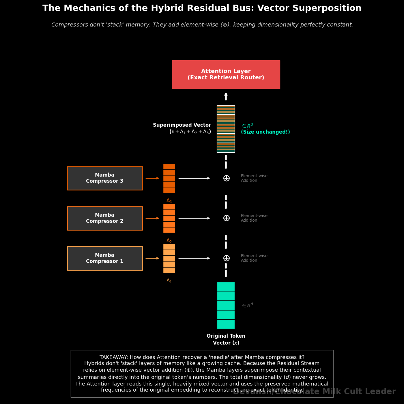
This is why hybrids don’t collapse into the same retrieval failure as pure SSMs or pure Linear Attention. The residual stream is a parallel data bus. The compressor layers write summaries onto it. They don’t erase what’s already there. The attention layer reads the full bus.
(Jamba uses this exact topology. Google’s RecurrentGemma does something slightly different — linear recurrence plus local sliding window attention — but the core KV-reduction goal and the residual-stream preservation mechanism are the same.)
How Much Memory Do Hybrid Transformers Actually Save?
Why did Jamba choose exactly 1 Attention layer for every 7 Mamba layers?
Because that’s roughly the ratio where the KV cache fits on one GPU and retrieval quality doesn’t collapse. The KV math tells you why fewer attention layers is better for memory. The needle survival distance tells you the minimum attention frequency before quality falls off a cliff. The 1:7 ratio sits in the overlap zone. Whether it’s the actual Pareto-optimal point or just the ratio AI21 shipped is a question the published ablation data doesn’t fully answer. So treat 1:7 as a validated existence proof, not a universal constant. If you’re designing your own hybrid, you’ll need to sweep this ratio against your own benchmark suite.
The memory math, however, is exact. And it’s where this gets fun.
Let’s bring back our KV cache formula from Part 1. The total bytes added to the cache per token is:
Delta_KV = 2 * L_attn * g * d_k * B_kv
(Where g is the number of KV heads after GQA, and d_k is the dimension per head.)
L_attn. That’s the variable that matters. In a pure Transformer, L_attn equals L — every layer caches Keys and Values. In Jamba, L_attn is L / 8. One-eighth. That single substitution changes everything downstream.
Let’s make it concrete. Imagine a 50B-class MoE model (50 billion total stored parameters, not active). 64 total layers, 8 KV heads, head dimension of 128, FP16 precision.
Model Weights: 50B MoE at INT4 quantization, roughly 25 GB of VRAM.
Pure Transformer KV Cache: At 256,000 tokens, a full 64-layer KV cache runs 2 * 64 * 8 * 128 * 256,000 * 2 bytes. That comes out to about 67 GB.
Now add it up. Weights (25 GB) + KV cache (67 GB) + framework overhead (~6 GB) = 98 GB.
The H100 has 80 GB of VRAM.
98 is bigger than 80. Now some of you are product managers and MBAs, so that assertion is likely a bit difficult to understand. No matter, take a second and really understand that for yourself. Ask ChatGPT if you have to. Once you understand this statemment we can proceed.
Your problem is simple — the model doesn’t fit (that’s what she said). You are forced into Tensor Parallelism across two GPUs, which instantly halves your gross margins and doubles your CAPEX. One variable — L_attn — is the reason your CFO is about to have a very bad quarter. Every single layer in that stack is demanding its own slice of the KV cache, and the cache does not negotiate. It takes its bytes or the model doesn’t run.
What if we instead apply the Hybrid ratio?
Hybrid KV Cache: 8 attention layers instead of 64. Cache drops from 67 GB to about 8.3 GB.
But we’re honest here, so we have to price the thing the pure Transformer didn’t pay for: the compressor states. Mamba recurrent states across 56 layers, d_model = 8192, d_state = 16, FP16: that’s 56 * 8192 * 16 * 2 bytes. Roughly 14.7 MB per user. Negligible. Basically, a rounding error on a GPU that thinks in gigabytes.
Swap in Linear Attention compressors instead, and it gets heavier: 56 layers, each with a (d_k * d_k) fast-weight grid per head, h = 64 heads, d_k = 128. That’s 56 * 64 * 128 * 128 * 2 bytes. Roughly 117 MB per user. About 14x the Mamba state. Still dwarfed by the 58.7 GB you saved on the KV cache, but large enough that your capacity planner had better know about it.
Hybrid total (Mamba compressor): Weights (25 GB) + Hybrid KV Cache (8.3 GB) + Mamba States (~0.015 GB) + Overhead (6 GB) = roughly 39.3 GB.
One GPU. 40 GB of headroom to spare for concurrency. By strategically deleting 87% of the attention layers, they crossed a hard hardware boundary that the pure Transformer couldn’t. The model that broke the H100 at 256K tokens now fits comfortably with room for dozens of concurrent users.
That’s the sell. Now let’s talk about why it’s harder than it sounds.
Why Isn’t Everyone Using Hybrid Transformers?
If Hybrids give you selective exact recall and the capacity of an SSM, why hasn’t the entire industry abandoned pure Transformers for them?
Three friction points. They don’t hurt equally.
1. What Happens When Hybrid Transformers Switch Kernels Mid-Forward Pass?
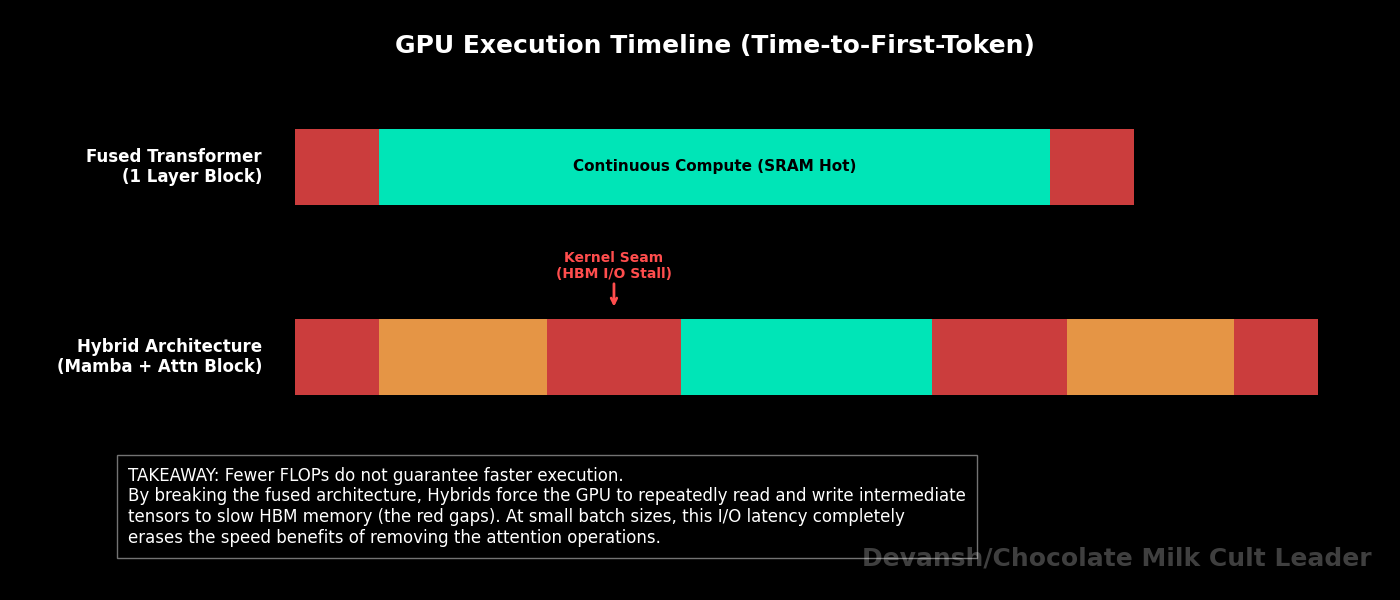
Modern GPUs hate context switching. High utilization means launching a massive, fused CUDA kernel and leaving data in the ultra-fast SRAM for as long as possible.
FlashAttention is a masterclass in this. It keeps tiles of Q, K, V in SRAM, computes the softmax and output projection without ever writing the n * n attention matrix to HBM, and achieves arithmetic intensities in the range of 100 to 200 FLOP/byte. Data stays hot. Math stays cheap relative to memory movement. Beautiful.
Hybrids wreck this by constantly crossing architectural seams. Run an associative scan (Mamba kernel). Write the activation tensors back to HBM. Launch a FlashAttention kernel. Read the tensors back into SRAM. Compute. Write back to HBM. Every seam crossing is a forced round-trip through HBM for activation tensors that scale as O(batch * seq * d_model) bytes.
Let’s price the damage on an H100 (3.35 TB/s HBM bandwidth):
Single activation tensor at batch=32, seq=4096, d=8192 in FP16: 32 * 4096 * 8192 * 2 * 2 = roughly 4.3 GB of bandwidth per seam crossing.
Eight seams across 64 layers (one per Jamba block) = ~34 GB of pure memory-movement overhead per forward pass that a fused Transformer never pays.
Effective arithmetic intensity at the seams craters to 10 to 30 FLOP/byte. Bandwidth-bound territory on every GPU shipping today.
You saved FLOPs by removing attention layers. You spent bytes switching between kernel types. The ledger doesn’t always net positive on wall-clock time.
This is the part that kills me about the hybrid discourse. Everyone celebrates the FLOP reduction. Nobody talks about the memory bus. You can have the most elegant architecture ever designed on paper, and the H100 will still punish you for making it read the same tensor twice. The silicon doesn’t care about your paper’s abstract. It cares about bytes moved per second, and you just asked it to move 34 GB of bytes it didn’t have to move before.
This is the great lie of the ArXiv preprint. On paper, Hybrids are the ultimate two-way player — they have the memory footprint of an SSM and the precision of a Transformer. In theory, Hybrids are your Mighty Mouse, with world-class striking AND world-class grappling. In reality, they’re closer to Kevin Lee, which get gas out hard in the transitions, leaving everyone struggling to see where Hybrids fit into the picture. You saved FLOPs by deleting attention layers, but you spent all those savings gasping for air on the memory bus while the H100 violently punishes you for context-switching
2. Why Can’t vLLM Serve Hybrid Transformers Out of the Box?
vLLM’s superpower is PagedAttention — it treats the KV cache like an operating system treats virtual memory, breaking it into non-contiguous blocks to eliminate fragmentation waste. Elegant, well-tested, the reason most production APIs can serve Transformers at reasonable cost.
A Hybrid breaks the assumption PagedAttention was built on: that the only per-request state is a KV cache. Hybrids have a growing KV cache (attention layers) and fixed-size recurrent states — whether those are Mamba’s d_model * d_state vectors (~0.26 MB per layer per user) or the massive Linear Attention fast-weight grids (~2.1 MB per layer per user, roughly 52 MB total across 25 compressor layers at the scale we priced in Section 3). Two completely different memory pools. Completely different growth dynamics. The KV cache grows linearly with tokens. The recurrent states are fixed but must be swapped in and out as requests get scheduled and preempted.
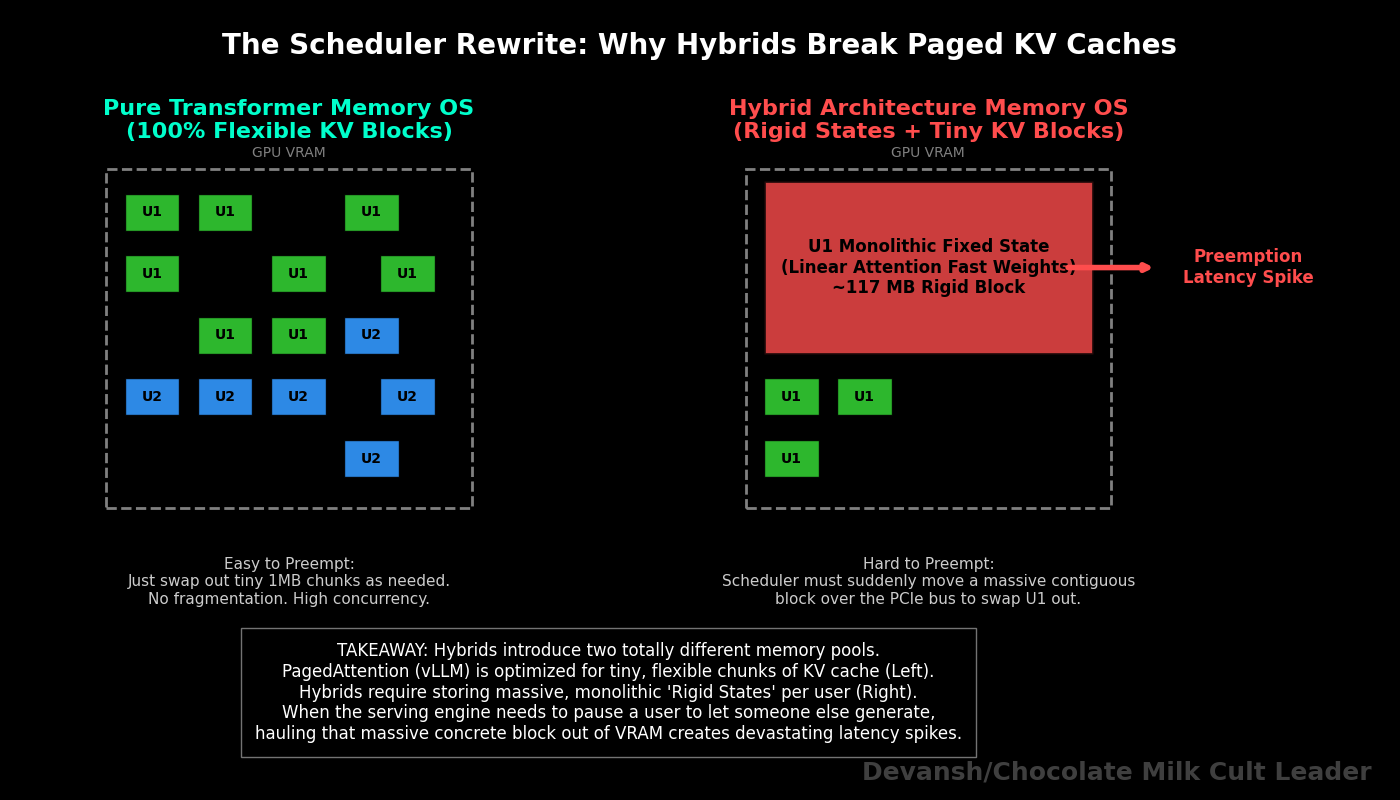
Building a memory allocator that pages KV blocks while simultaneously managing Mamba state swaps or Fast-Weight grid swaps is a scheduler rewrite. Work has been done to serve these, but it’s still not as stable as normal transformers.
For most serving teams, this is the actual deployment barrier. After all, the real question is not whether the model works. Lots of things work in a benchmark lab. The real question is whether your serving stack can carry it without needing therapy
And if the answer is no, the FLOP savings don’t matter. You’re not shipping. The model sits on your benchmarking cluster looking beautiful while your competitors serve worse models to paying customers.
3. Do Hybrid Transformers Actually Remove the Memory Wall?
No.
Hybrids shrink L_attn. But L_attn is still greater than zero. The KV cache still grows linearly with n. You haven’t removed the wall. You’ve reduced the slope of the line.
Dividing the cache by 8 at 256K tokens pushes the memory wall back by roughly 8x. Your 256K limit becomes a ~2M token limit before you hit the same overflow.
But does 8x actually hold? Only if the compressor states stay negligible at scale.
Mamba compressors: recurrent states are still 14.7 MB per user at 2M tokens. Fixed-size, unchanged. The 8x ceiling holds clean.
Linear Attention compressors: fast-weight grids are still 117 MB per user. Also fixed-size. But at 100 concurrent users, that’s 11.4 GB of VRAM just for compressor states — no longer a rounding error. The effective multiplier drops from 8x to something closer to 6 to 7x depending on your concurrency target.
Compressor states don’t grow with context. They grow with concurrency. At high user counts, the “fixed-size” advantage partially unwinds because you’re paying that fixed cost per user. And if you’re running a high-concurrency production API (which is… everyone who’s trying to make money on this), the wall moved less far than the napkin math suggested.
This is the tragedy of every “efficient” architecture. You solve one constraint, and another one tightens. The memory wall was context-bound, so you made it concurrency-bound instead. You didn’t escape the physics. You rotated the axes of the problem and hoped the new orientation was more survivable. Sometimes it is. But the wall is still there, waiting to Yamcha you.
Hybrids are the sharpest engineering compromise in the industry right now. Bridge technology. They push the memory wall back far enough to make current enterprise use cases viable at current hardware prices. But they do not remove the wall.
To actually survive beyond the 1-million-token limit without sacrificing exact recall, we have to look away from the architecture of the model entirely, and look at the architecture of the data center.
That brings us to Distributed Exact Attention.
Section 5: Extreme Context (Changing the Data Center)
Hybrids are an elegant compromise. They delay the memory wall by shrinking the KV cache. But maybe elegance is not your problem; maybe you’re stubborn, or rich, or both
So, what if you refuse to compromise? What if you are building an agentic workflow that reads a 1-million-token codebase, and you absolutely cannot afford the feature collision of an SSM or the retrieval loss of Linear Attention? You want the pure, unmodified, O(n²) global exact recall of a Transformer.
If you won’t change the architecture of the model, you have to change the architecture of the data center.
This brings us to Context Parallelism and algorithms like Ring Attention.
What Does a 1-Million-Token Sequence Actually Cost?
Let’s price out exactly what a 1-million-token sequence costs in memory. We will use a 70B-class model as our proxy, assuming 80 layers, Grouped Query Attention with 8 KV heads, a head dimension of 128, and FP16/BF16 precision (2 bytes).
The KV cache formula: Layers * KV Heads * Head Dim * Tokens * 2 (for K and V) * 2 bytes. 80 * 8 * 128 * 1,000,000 * 2 * 2 = ~328 GB.
The KV cache for a single request is roughly 328 GB. Not the model. Not the activations. Not the optimizer states. Just the cache. One user’s context window.
Common high-end enterprise deployments run 80 GB H100s. A single H100 cannot hold this request. Four H100s cannot hold this request. You need a minimum of 5 GPUs just for the KV cache alone, before you even load the model weights. At on-demand H100 pricing (~$3/GPU/hour), that’s $15/hour just to remember what one user said. And you haven’t done any math yet. Just like these new age transcription tools, you’re going to be a lot of money just to not forget; even before the cost of intelligence curb stomps you later.
Standard Tensor Parallelism solves weight capacity, and it scales well inside a single server node where 8 GPUs are connected by ultra-fast NVLink (~900 GB/s bidirectional). But TP’s all-reduce synchronization costs grow painfully once your memory requirements force you to cross the node boundary onto InfiniBand (~50 GB/s per link). That’s an 18x bandwidth cliff between “inside the box” and “across the wire.”
To survive 1 million tokens across a massive cluster without bottlenecking on weight syncs, you must partition the sequence itself.
How Does Ring Attention Distribute Context Across GPUs?
The core idea comes from “Ring Attention with Blockwise Transformers for Near-Infinite Context”: instead of partitioning the model’s weights across devices (which is what Tensor Parallelism does), partition the sequence. Each GPU gets a shard of tokens and handles its own slice of the attention computation.
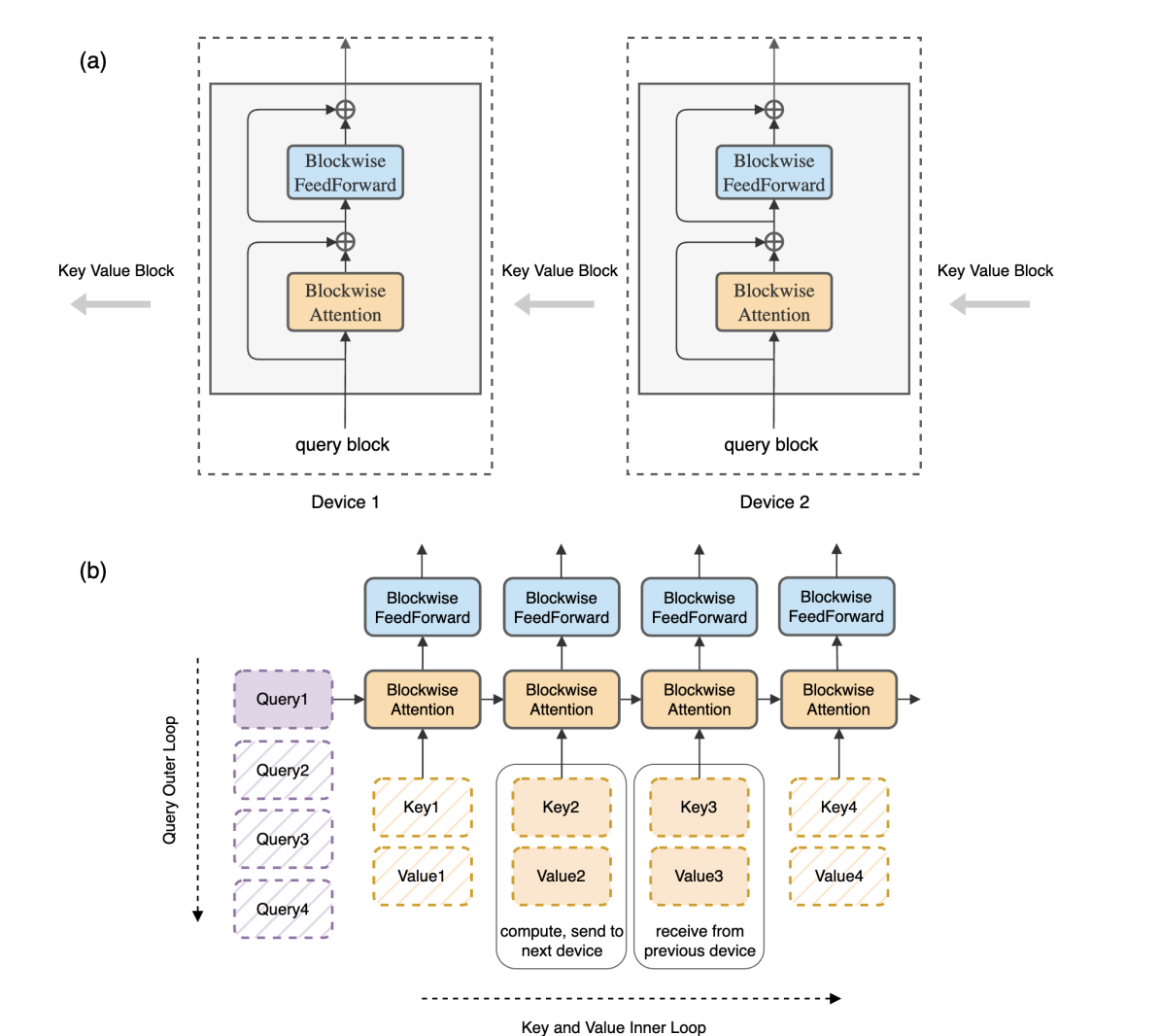
Let’s say we have p devices. We take our 1-million-token sequence and chop it into p shards. Each GPU is now responsible for n/p tokens.
The local compute per device drops drastically. Instead of calculating a massive (n * n) attention grid, each GPU calculates a smaller local block. But attention requires global interaction — for causal attention, each device must eventually incorporate all relevant causal predecessors for the tokens in its shard. That means pulling remote KV blocks from other devices over the network.
If a GPU simply stops computing to wait for a 40 GB block of KV cache to arrive over an Ethernet cable, your cluster dies.
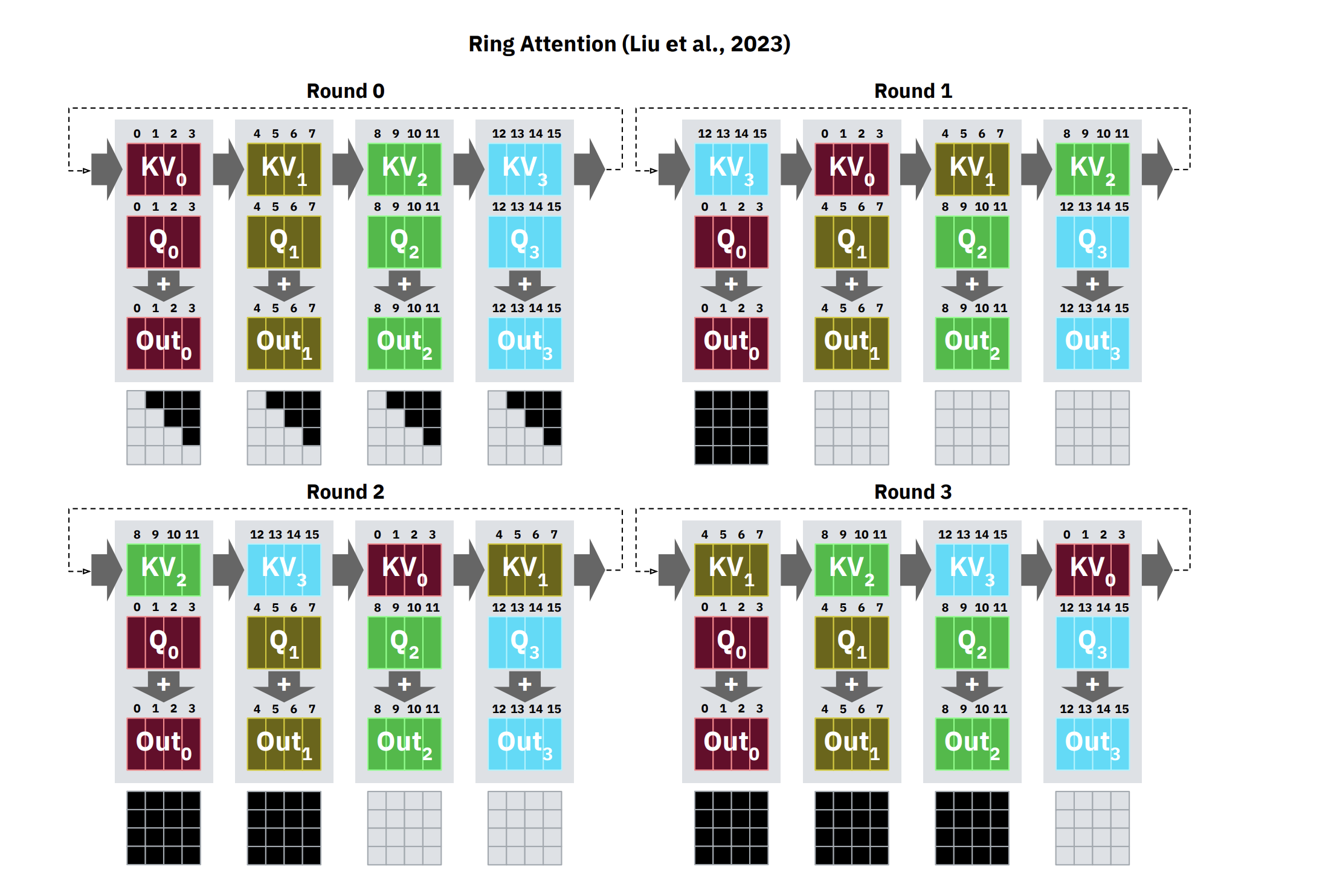
Ring Attention solves this by arranging the GPUs in a logical ring and overlapping communication with computation:
A GPU starts computing the attention scores for its local Q block against whatever K, V block it currently holds.
At the exact same time, it sends its K, V block to the next GPU in the ring and begins receiving a different K, V block from the previous GPU.
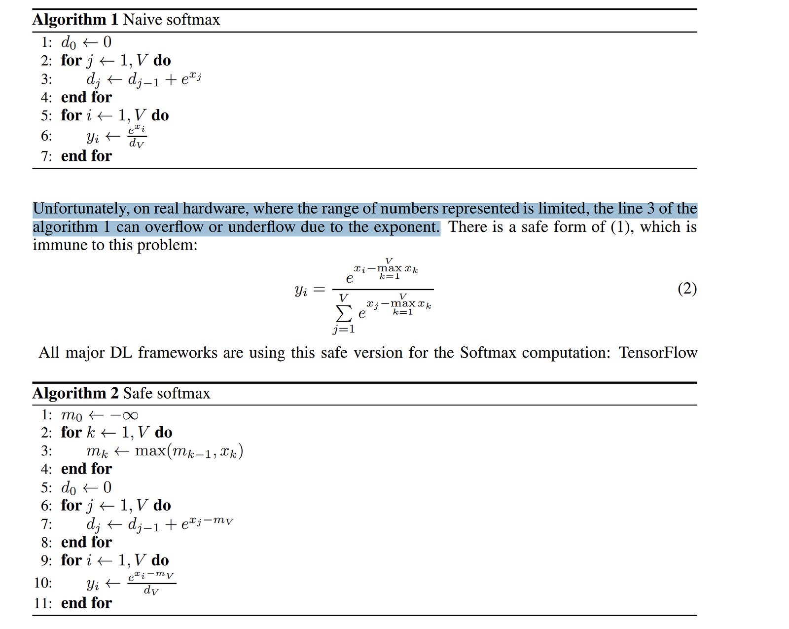
After p-1 such passes, every GPU has seen every other GPU’s K, V block. The full attention output is assembled via blockwise accumulation that preserves numerical correctness (using the online softmax trick from “Online Normalizer Calculation for Softmax”).
Why a ring specifically, and not all-to-all communication? Because a ring minimizes concurrent network transfers to exactly 1 send + 1 receive per device per step. All-to-all would require every device to simultaneously blast its KV block to every other device, saturating the network instantly. The ring topology is the minimum-bandwidth schedule that achieves full coverage.
The key condition that makes this work: if the time to compute the local attention block is longer than the time to transfer the KV block to the next device, communication is fully hidden. The math runs while the bytes move. Zero overhead. In theory.
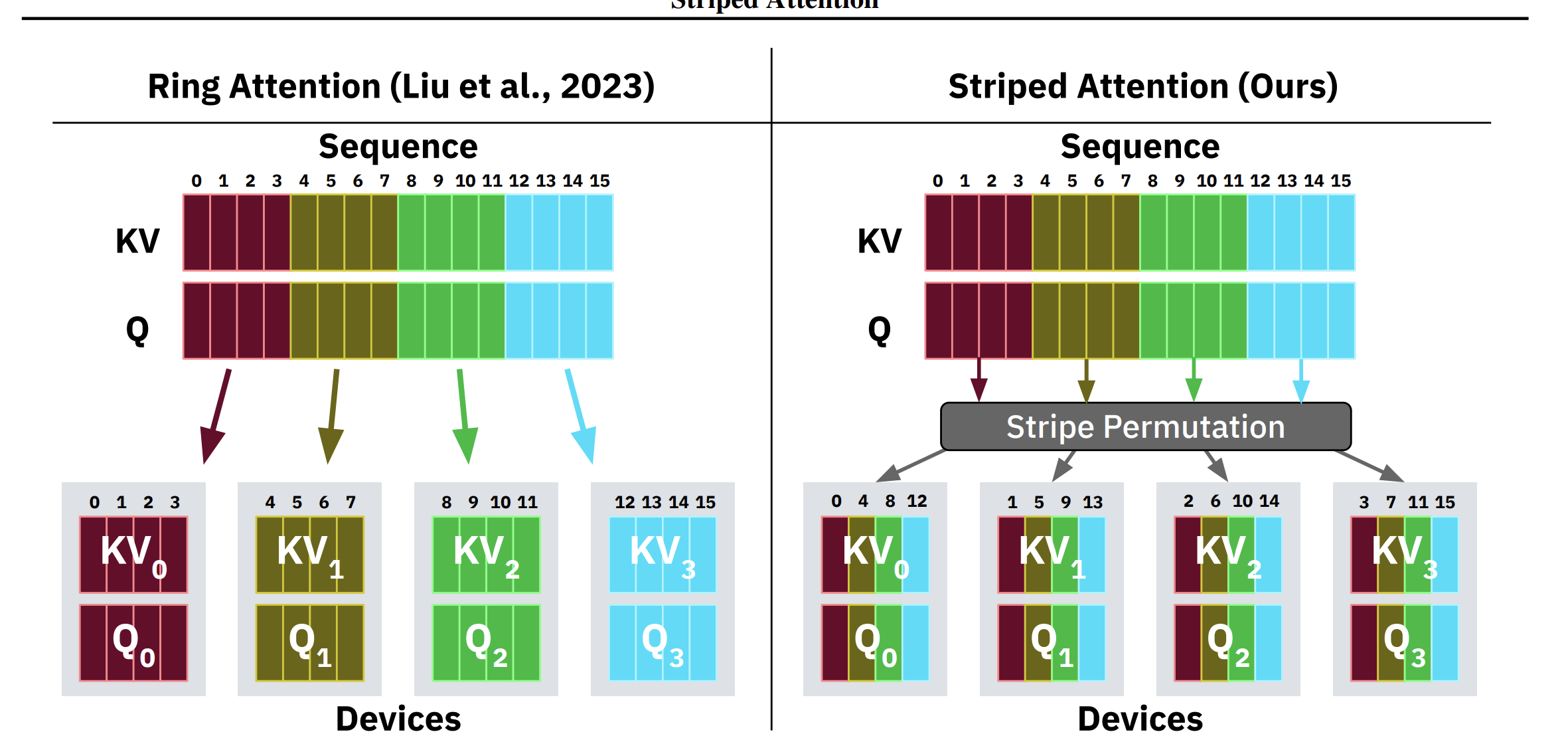
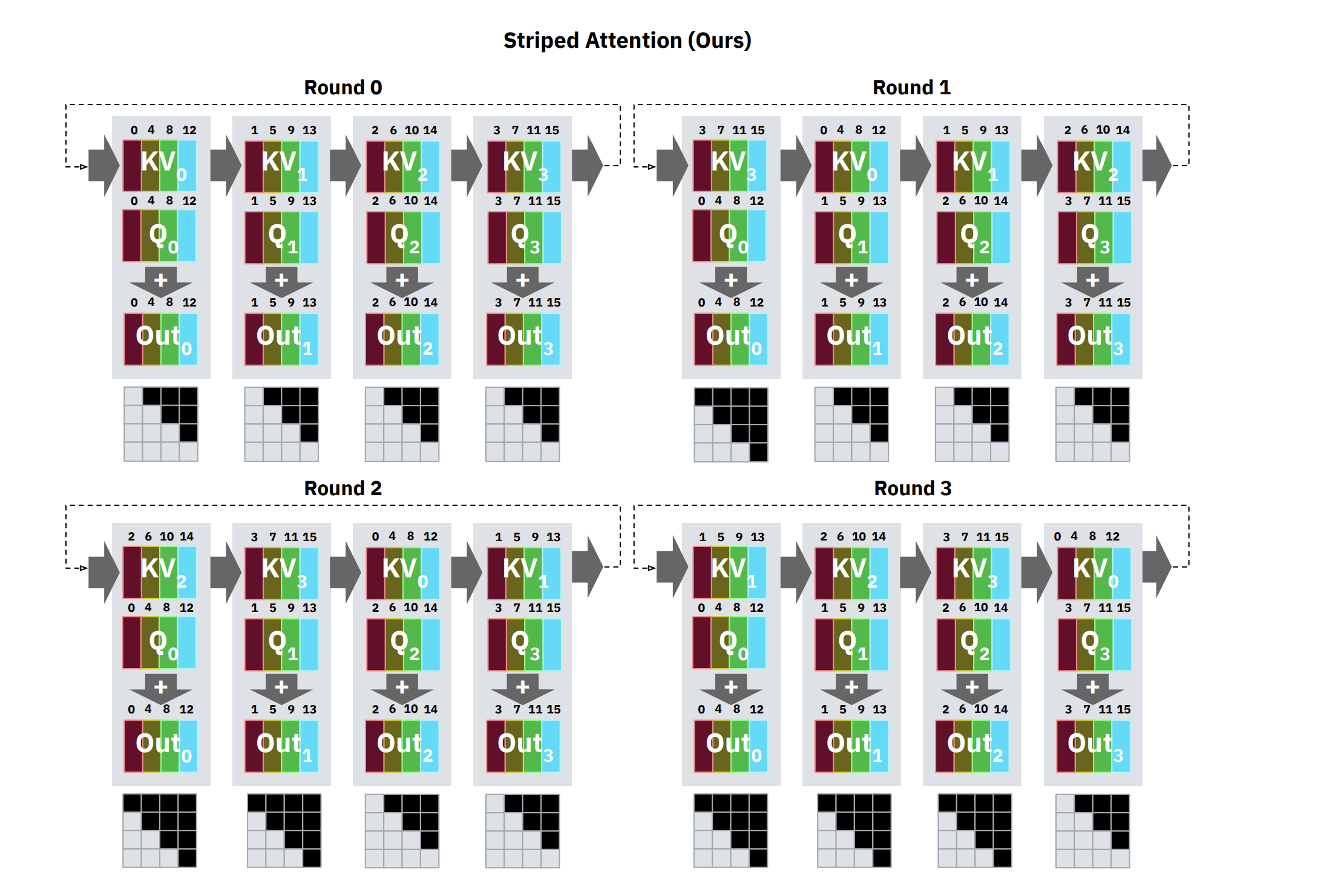
There’s a subtle but important problem with naive Ring Attention that “Striped Attention: Faster Ring Attention for Causal Transformers” identified: causal masking creates severe load imbalance. In causal (autoregressive) attention, the attention matrix is triangular — early tokens attend to few predecessors, late tokens attend to many. If you assign contiguous subsequences to each device, the device holding the last tokens does far more work than the device holding the first tokens. Everyone else sits idle waiting for the slowest device to finish.
Striped Attention fixes this by distributing tokens in a round-robin pattern (device 0 gets tokens 0, p, 2p, …; device 1 gets tokens 1, p+1, 2p+1, …). This spreads the triangular workload evenly. The result: up to 1.45x end-to-end throughput improvement over vanilla Ring Attention on causal models.
Why Does Ring Attention Break Down During Decode?
In prefill, you are processing massive blocks of tokens simultaneously. The arithmetic intensity is enormous — thousands of FLOPs for every byte of data. The compute takes a long time relative to the network transfer. Because the compute is slow, the network has plenty of time to quietly pass the KV blocks in the background. The overlap condition holds comfortably.
Let’s make this concrete with the numbers from Meta’s “Context Parallelism for Scalable Million-Token Inference” paper. They report processing a 1-million-token prefill on Llama 3 405B in 77 seconds across 16 nodes (128 H100 GPUs), achieving 93% parallelization efficiency and 63% FLOPS utilization. That’s near-linear scaling for prefill. The overlap condition holds because each device is grinding through enormous local attention blocks that take long enough to fully mask the inter-node transfers.
But if you’ve been reading our guides on inference, you know that inference has another stage, the decode. So, what happens during Decode?
In decode, you generate tokens one by one. One token means one query vector. The local attention computation for a single query against even a large KV block finishes almost instantly — the arithmetic intensity craters. But you still have to pass the KV blocks around the ring to compute global attention for that one new token.
Let’s price the mismatch. For a single decode step on one device:
Compute: One query vector (d_k = 128 floats) dot-producted against n/p key vectors. For n = 1M tokens across p = 128 GPUs, that’s about 7,800 key vectors per device. The compute is roughly 2 * 7,800 * 128 = ~2 million FLOPs per head, times 128 heads = ~256 million FLOPs total. On an H100 doing ~990 TFLOPS (FP16), that takes roughly 0.26 microseconds.
Transfer: The KV block that needs to move to the next device is n/p * d_k * 2 (K and V) * 2 bytes = 7,800 * 128 * 2 * 2 = ~4 MB per head group. Across all KV head groups with GQA: ~32 MB. On 400 Gb/s InfiniBand (~50 GB/s effective), that takes about 0.64 milliseconds.
The compute finishes in microseconds. The transfer takes milliseconds. The overlap condition is destroyed by a factor of roughly 2,500x. The GPUs finish their math and sit idle, waiting for the network.
This is the physical bandwidth hierarchy working against you:
GPU HBM bandwidth: ~3,350 GB/s
Intra-node NVLink: ~900 GB/s
Inter-node InfiniBand: ~50 GB/s
During decode, you have successfully moved the bottleneck off the ultra-fast HBM and placed it directly onto the network cable. Your generation speed becomes constrained by interconnect bandwidth, not GPU math. According to the “Context Parallelism” paper, CP is “best suited for improving prefill performance” and decode latency regresses under it.
What Is StreamingLLM and How Do Attention Sinks Work?
If you don’t have a multi-node InfiniBand cluster to run exact distributed attention, but you still need to process infinite context (like a 24/7 ambient voice assistant), there is one final, ruthless architectural hack: just delete the middle.
If you allow a KV cache to grow infinitely, the GPU crashes. But researchers noticed that if you just naively evict the oldest tokens when the cache gets full (a rolling window), the model completely collapses. Perplexity explodes. Not gradual degradation — catastrophic failure.
Why? Because of Attention Sinks.
“Efficient Streaming Language Models with Attention Sinks” discovered the mechanism. Under autoregressive causal attention, early tokens become persistent global anchors that absorb surplus attention mass. The reason traces directly to the interaction between causal masking and softmax normalization.
Here’s the first-principles chain: in causal attention, token 1 is visible to every subsequent token. Token 2 is visible to all but one. Token 1000 is only visible to tokens after position 1000. This asymmetry means early tokens accumulate vastly more gradient signal during training than late tokens — they participate in every attention distribution in the sequence. The model adapts to this by learning to dump “excess” attention probability onto these early tokens, effectively using them as a numerical pressure valve for the softmax normalization.
It’s not that the first tokens contain important information. The “Attention Sinks” paper showed this explicitly: you can replace the first four tokens with newline characters (“\n”) and the model still recovers. The tokens themselves are semantically irrelevant. What matters is their position — they’ve become structural load-bearing elements of the attention distribution, regardless of content.
If you delete those sink tokens, the softmax budget loses its pressure valve. The remaining attention scores destabilize because the distribution they were trained to produce no longer sums correctly without the sinks absorbing the overflow. The whole thing collapses.
The fix is StreamingLLM. You keep the KV cache strictly bounded to a fixed size (e.g., 4,000 tokens). You permanently lock a small number of sink tokens (the first 4 words) into the cache so the softmax math stays stable. Then you use the remaining slots as a rolling window for the most recent tokens.
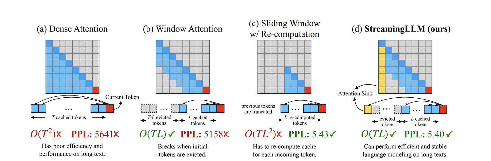
Everything in the middle is permanently thrown away.
This gives you a perfectly flat, O(1) memory footprint. The “Attention Sinks” paper demonstrated it running stable on Llama-2, MPT, Falcon, and Pythia at up to 4 million tokens with zero degradation in perplexity — and 22.2x speedup over sliding window recomputation. It runs infinitely with no latency growth.
But once again, the fundamental law holds: you paid for your flat memory footprint with precision. The model has zero memory of anything that fell outside the rolling window. If a critical fact appeared at token 50,000 and the window only holds the last 4,000, that fact is gone.
In other words, StreamingLLM is not a context extension method. It’s a context amputation method that keeps the patient alive.
We’ve covered a lot of techniques here. So, to end, let’s break down the costs better.
Section 6: What are the Costs of the Different Transformer Variants?
We have spent five sections tearing apart the linear algebra of the Transformer, the differential equations of Mamba, the associative math of Linear Attention, and the bandwidth limits of InfiniBand.
Theoretical discussions are nice, but deployment is a physical game of fit. You either have the VRAM to serve 1,000 concurrent users, or you go bankrupt paying $2.50/hour for an H100 that is serving 4 people. Every equation we derived in this series terminates in the same place: a line item on someone’s cloud bill, a number of users per GPU, a price per token.
To see exactly how the “Quadratic Tax” destroys margins — and to prove why the escape routes we just covered are existentially necessary — we are going to run a stress test.
What Are the Constraints of Our Stress Test?
We will assume a standard 80 GB NVIDIA H100. We subtract a strict 6 GB overhead for the runtime, memory allocators, and temporary activations. That leaves us roughly 74 GB of usable VRAM.
We will test three proxy models at INT4 weight quantization (to maximize the space left for the cache):
1B Model (d = 2048, L = 16, g = 8, d_k = 64). Weights: ~0.6 GB at INT4.
3B Model (d = 3072, L = 24, g = 8, d_k = 128). Weights: ~1.8 GB at INT4.
70B Model (d = 8192, L = 80, g = 8, d_k = 128). Weights: ~35 GB at INT4.
We will use INT8 quantization for the KV cache (1 byte per number).
The KV cache formula, carried forward from Part 1:
KV bytes per user = L * g * d_k * n * 2 (K and V) * B_kv
Where L is layers, g is KV head count, d_k is head dimension, n is context length, and B_kv is bytes per value (1 byte for INT8). Let’s sanity-check one cell before we trust the numbers: for the 70B model at 128K context, that’s 80 * 8 * 128 * 128,000 * 2 * 1 = 20,971,520,000 bytes = ~20.97 GB. One user. Just the cache.
How Does KV Cache Size Scale With Context Length?
Watch what happens to the KV cache per user (INT8 quantization) as we stretch context from 4K to 1 million tokens.
1B model (weights: ~0.6 GB): 4K = 0.07 GB. 32K = 0.52 GB. 128K = 2.10 GB. 1M = 16.38 GB. The cache at 1 million tokens is 27x larger than the model itself. The thing that stores the context has completely consumed the machine that does the thinking.
3B model (weights: ~1.8 GB): 4K = 0.20 GB. 32K = 1.57 GB. 128K = 6.29 GB. 1M = 49.15 GB. At 128K context, the cache is already 3.5x the weight of the model. At 1M, a single user’s cache eats 60% of the entire H100.
70B model (weights: ~35 GB): 4K = 0.66 GB. 32K = 5.24 GB. 128K = 20.97 GB. 1M = 163.84 GB. The H100 only holds 80 GB. At 1 million tokens, a single user’s KV cache is twice the size of the entire GPU. You are physically dead in the water before you load the first weight.
How Does Context Length Destroy Concurrency?
The size of the cache dictates your batch size. Every user gets their own cache. Divide your remaining VRAM (after weights and overhead) by the per-user cache size, and you get the absolute hardware ceiling for concurrent users on a single 80 GB H100 (INT4 weights, INT8 KV cache).
1B model: 4K = ~1,112 users. 32K = ~140 users. 128K = ~35 users. 1M = ~4 users.
3B model: 4K = ~366 users. 32K = ~46 users. 128K = ~11 users. 1M = ~1 user.
70B model: 4K = ~59 users. 32K = ~7 users. 128K = ~1 user. 1M = doesn’t fit.
This is the Concurrency Collapse that Part 1 warned you about.
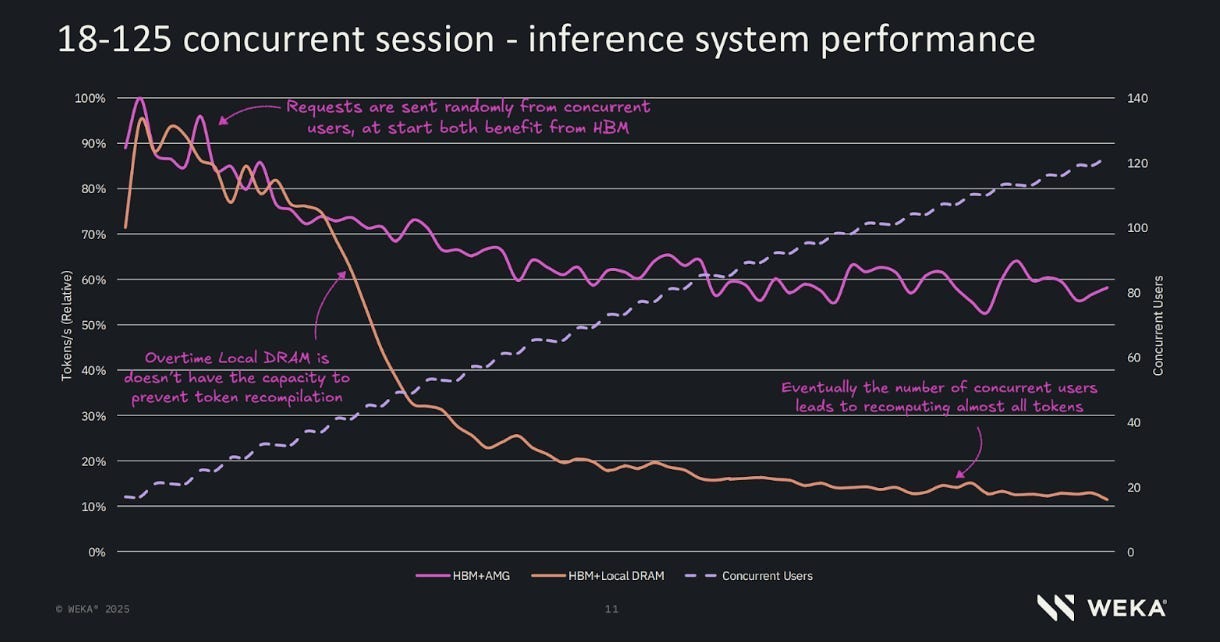
If you run a 70B model at 4K context, you can fit 59 concurrent users on a single H100. At $2.50/hour, your per-user hardware cost is roughly $0.04/hour. Highly profitable. The kind of unit economics that makes a VC’s eyes glaze over with dollar signs.
If you offer a 128K context feature, you can fit exactly 1 user on that GPU. Your hardware cost instantly spikes to $2.50/hour per user. You haven’t changed the model. You haven’t changed the hardware. You just changed the context length, and your unit economics became 59x more expensive.
That’s not a scaling problem. That’s a business model collapse. And it explains why every API provider prices long-context requests at a steep premium — they’re not gouging you, they’re passing along the physical cost of the quadratic tax on their KV cache.
Let’s convert this to the number your finance team actually cares about. Assume each user generates ~500 output tokens per request at ~50 tokens/second (10 seconds of generation), and the GPU runs at 70% utilization (most LLMs would probably run a bit faster, but they also consume more thinking tokens/deal with memory + will have input/output processing for your app, so this is a reasonable set of params for quick math).
At 4K context, 70B model: 59 users * 500 tokens * 3600/10 seconds * 0.7 utilization = ~7.4M output tokens/hour. At $2.50/hour GPU cost (mid-range cloud rate), that’s roughly $0.34 per million output tokens in raw hardware cost. The retail API price for a model this size is $3–25/M depending on provider — which means at short context, inference margins are enormous. The hardware cost is a rounding error on the price you charge.
At 128K context, 70B model: 1 user * 500 tokens * 3600/10 * 0.7 = ~126K output tokens/hour. At $2.50/hour, that’s roughly $19.84 per million output tokens in raw hardware cost alone. That is higher than what Claude and OpenAI charge retail. You aren’t running a SaaS startup anymore; you are running a philanthropic foundation that yeets VC dollars to your cloud provider just so one power-user can summarize a PDF they aren’t even going to read.
And that’s before you account for the prefill cost on the 128K input.
This is why long-context inference is the single most important economic problem in AI infrastructure today. Because the money doesn’t work at scale.
How Do the Escape Routes Change These Numbers?
Now let’s apply the architectural escape routes we spent this article dissecting. Take the worst case from our numbers: the 70B model at 128K context, currently fitting 1 user on an H100 with a 20.97 GB KV cache.
Escape Route 1: Low-Rank KV Compression / MLA (Section 1)
In our earlier section on KV cache optimization, we covered DeepSeek-V2’s Multi-head Latent Attention. Instead of caching the full Key and Value tensors, MLA projects each token down to a compressed latent vector and reconstructs the Keys and Values on the fly during attention. The 2 * g * d_k storage term gets replaced by a much smaller compressed dimension d_c.
DeepSeek reported a 93.3% reduction in KV cache size. Applied to our 70B scenario:
New KV cache: 20.97 GB * 0.067 = ~1.40 GB per user.
Concurrency: (74 GB — 35 GB weights) / 1.40 GB = ~27 users.
$/M output tokens: drops from $19.84 to roughly $0.73.
What you lost: Compute. Reconstructing Keys and Values from the compressed latent requires an extra matrix multiplication every decode step — you’re trading memory capacity for arithmetic intensity. And the compression breaks standard RoPE position embeddings, forcing you into decoupled RoPE strategies that add implementation complexity. The quality numbers hold if the compression rank is chosen carefully. If you get greedy and compress too aggressively, retrieval precision degrades the same way it does in any lossy compression scheme.
Escape Route 2: Hybrid Transformers (Section 4)
Jamba-style architecture: 1 Attention layer for every 7 Mamba layers. L_attn drops from 80 to 10.
New KV cache: 10 * 8 * 128 * 128,000 * 2 * 1 = ~2.62 GB per user. Plus Mamba recurrent states across 70 layers: ~14 MB per user, negligible.
Concurrency: (74 GB — 35 GB weights) / 2.62 GB = ~14 users.
$/M output tokens: drops from $19.84 to roughly $1.42.
What you lost: Exact recall only fires at every 8th layer. Tasks requiring verbatim retrieval — citation, code search, legal discovery — degrade depending on needle survival distance. Your serving stack needs a 2–4 month scheduler rewrite for the dual memory pool (Section 4). Kernel switching overhead eats ~10–15% of your theoretical FLOP savings at the architectural seams. And you’re retraining or fine-tuning from a Hybrid checkpoint, which means weeks of GPU time before you can even start serving.
Escape Route 3: Pure Mamba / Linear Attention (Sections 2 & 3)
Rip Attention out entirely. The KV cache drops to zero. Replace it with a fixed recurrent state (Mamba) or a fixed fast-weight grid (Linear Attention, ~52 MB as priced in Section 3).
Per-user state: ~20 MB (Mamba) or ~168 MB (Linear Attention at this model scale — 80 layers, 64 heads, d_k = 128).
Concurrency with Mamba: (74 GB — 35 GB weights) / 0.020 GB = theoretically ~1,950 users. In practice you hit compute throughput limits long before memory limits. But memory is no longer the binding constraint at any context length. That alone changes the entire economics.
Concurrency with Linear Attention: (74 GB — 35 GB) / 0.168 GB = ~232 users.
$/M output tokens: craters to fractions of a cent on the hardware side.
What you lost: Exact retrieval. A pure Mamba model at 128K context cannot do needle-in-haystack with the same precision as full Attention. Feature collision degrades with sequence length — the longer the context, the worse the compression artifacts get. For workloads requiring verbatim recall (legal, code, medical records), this is a categorical capability loss, not a slight quality tradeoff. You also need a full retrain from scratch on the new architecture, thinner ecosystem tooling, fewer battle-tested serving frameworks, and custom CUDA kernels that are sensitive to quantization drift (Section 2).
Escape Route 4: Distributed Exact Attention (Section 5)
Refuse to compromise on recall. Shard the sequence across multiple GPUs using Ring Attention / Context Parallelism. Keep the full, unmodified O(n²) attention.
Spread the 21.47 GB KV cache across p = 4 GPUs (staying within a single node on NVLink). Each device holds ~5.4 GB of cache. With model weights distributed via TP4, each GPU holds ~8.75 GB of weights.
Per-device memory: 8.75 GB weights + 5.2 GB cache + overhead = ~20 GB. Fits comfortably on an 80 GB H100 with room for multiple users per device.
Concurrency per 4-GPU node: roughly ~10 users.
What you gained: Perfect recall. Zero quality loss. The exact same model, distributed differently.
What you lost: Prefill scales near-linearly. Decode becomes network-bound. Tokens-per-second per user during generation drops hard compared to single-GPU serving, because every decode step requires a KV block round-trip across devices. NVLink within a node (~900 GB/s) is survivable. InfiniBand across nodes (~50 GB/s) is brutal.
Your $/M tokens doesn’t improve. It gets worse — you’re paying for 4 GPUs to serve the same users that 1 GPU handled at 4K context. The advantage is you can offer 128K context at all, which you physically couldn’t before. Revenue-enablement play, not cost reduction.
Escape Route 5: StreamingLLM (Section 5)
Bounded cache of ~4,000 tokens. Lock the first 4 sink tokens. Roll the window forward. Amputate the middle.
Per-user cache: 70B model at 4K effective window = ~0.66 GB (same as the 4K row in our original numbers).
Concurrency: back to ~59 users. Same as the 4K baseline.
What you gained: Infinite input length. Zero latency degradation. O(1) memory. The same economics as 4K context regardless of how long the conversation runs. 22.2x speedup over sliding window recomputation.
What you lost: Everything outside the window. If a user mentions something 50,000 tokens ago, it’s gone. For multi-turn chatbots where only the recent conversation matters, this works. For anything requiring full document recall, it’s useless.
What Does This All Mean?
We have hit the bottom of the stack. We traced the quadratic tax from the raw algebra of the Softmax function, to the exact byte size of the KV cache, to the arithmetic intensity of the SRAM, to the physical bandwidth of the network cables, and finally to the dollar cost per million tokens.
One law unifies every architecture we covered:
During generation, the bottleneck is bytes moved, not math computed.
Every architecture answers the same question differently: which bytes are you willing to not move?
Standard Attention moves all the bytes. Perfect recall. KV cache grows with n. Eventually crushes your concurrency and your margins.
MLA / Low-Rank Compression moves fewer bytes by compressing KV storage into a latent vector and reconstructing on the fly. You trade memory for compute and accept the engineering complexity of decoupled positional encodings.
Hybrids move fewer KV bytes by deleting most attention layers and compressing the rest through SSM or Linear Attention blocks. You gain concurrency, lose some retrieval precision, and inherit a serving infrastructure headache.
Mamba / Linear Attention move a fixed number of bytes regardless of context length. Memory stops being the binding constraint entirely. Retrieval quality degrades the longer the context gets.
Distributed Attention moves the bytes across network cables instead of memory buses. Perfect recall at any length. Prefill scales beautifully. Decode becomes a network bandwidth problem. You pay with hardware cost.
StreamingLLM moves almost nothing. Flat O(1) memory. Infinite input length. Everything outside the rolling window is amputated forever.
Conclusion: What Happens When You Don’t Have 80 GB of VRAM?
We started this series with a single matrix multiplication — Q times K-transpose — and traced its consequences all the way down to the dollar cost of serving one user. Along the way we broke open five architectures, priced every state tensor and cache entry in bytes, and watched each one solve the quadratic tax by sacrificing something else. Memory for precision. Precision for memory. Elegance for infrastructure complexity. The unifying law held at every layer of the stack: during generation, you are bottlenecked by the bytes you move, not the math you compute.
But every architecture we’ve covered was designed for the same environment: a data center rack with 80 GB H100s, terabytes-per-second memory bandwidth, and a power budget that nobody in the building actually tracks. The tradeoffs we mapped — KV cache vs. compression, exact recall vs. fixed state, FLOP reduction vs. kernel switching overhead — all assume you have that kind of silicon to trade with.
But the fastest-growing deployment surface for AI isn’t the data center. It’s the pocket.
An iPhone has 4–6 GB of shared RAM. A terrible memory bus compared to HBM. A battery that dies in hours under sustained compute. The Qualcomm NPU in a midrange Android phone has roughly 1/500th the memory bandwidth of an H100. On these devices, the entire premise of this article — that you can choose where to spend your memory budget — collapses, because there is no budget. There’s barely enough room to load the weights, let alone maintain any kind of per-user state.
The architectures that win in the cloud won’t survive on the edge. Transformers are too memory-hungry even with every optimization we covered. Hybrids still carry KV cache for their attention layers. Even Mamba’s recurrent state, negligible at data center scale, becomes a real constraint when your total VRAM is measured in single-digit gigabytes shared with the operating system, the display buffer, and whatever else the user has open.
Edge AI needs something different. And the companies building for it — Liquid AI resurrecting continuous-time neural networks, the xLSTM lineage pushing gated recurrences below 1B parameters, RWKV attempting to make linear attention work at mobile scale — are solving a constraint set that this article never touched: power per token, latency under thermal throttling, and inference quality at model sizes where every megabyte of state is a megabyte stolen from something else.
That’s the next subject of the deep dive. We’ll apply the same in-depth math and financial analysis to the scenario when silicon gets small, the power budget gets brutal, and the architectures that looked elegant in an 80 GB world start looking like the wrong tool entirely.
Thank you for being here, and I hope you have a wonderful day,
Dev <3
If you liked this article and wish to share it, please refer to the following guidelines.
That is it for this piece. I appreciate your time. As always, if you’re interested in working with me or checking out my other work, my links will be at the end of this email/post. And if you found value in this write-up, I would appreciate you sharing it with more people. It is word-of-mouth referrals like yours that help me grow. The best way to share testimonials is to share articles and tag me in your post so I can see/share it.
Reach out to me
Use the links below to check out my other content, learn more about tutoring, reach out to me about projects, or just to say hi.
Small Snippets about Tech, AI and Machine Learning over here
AI Newsletter- https://artificialintelligencemadesimple.substack.com/
My grandma’s favorite Tech Newsletter- https://codinginterviewsmadesimple.substack.com/
My (imaginary) sister’s favorite MLOps Podcast-
Check out my other articles on Medium. :
https://machine-learning-made-simple.medium.com/
My YouTube: https://www.youtube.com/@ChocolateMilkCultLeader/
Reach out to me on LinkedIn. Let’s connect: https://www.linkedin.com/in/devansh-devansh-516004168/
My Instagram: https://www.instagram.com/iseethings404/
My Twitter: https://twitter.com/Machine01776819
Thank you for such a great article. The level of detail is impressive—I even felt it was close to a survey paper. I liked it so much that I shared it with my colleagues.
Seems like the other path forward is split your context into parallel queries and recombine answers. Considering that (prompt-context-query) sandwich repeats prompt and query whole, but you can split many kinds of context which have no inherent serial dependencies, you might convert a 1MT problem into 8 150kT problems that can be merged with orchestration. Agents orchestrate extensively already, perhaps an economical path forward.