
The Future of On-Device AI
How Liquid AI built the Best Edge AI Model in the World. And what this reveals about the next wave of model design.

It takes time to create work that’s clear, independent, and genuinely useful. If you’ve found value in this newsletter, consider becoming a paid subscriber. It helps me dive deeper into research, reach more people, stay free from ads/hidden agendas, and supports my crippling chocolate milk addiction. We run on a “pay what you can” model—so if you believe in the mission, there’s likely a plan that fits (over here).
Every subscription helps me stay independent, avoid clickbait, and focus on depth over noise, and I deeply appreciate everyone who chooses to support our cult.
PS – Supporting this work doesn’t have to come out of your pocket. If you read this as part of your professional development, you can use this email template to request reimbursement for your subscription.
Every month, the Chocolate Milk Cult reaches over a million Builders, Investors, Policy Makers, Leaders, and more. If you’d like to meet other members of our community, please fill out this contact form here (I will never sell your data nor will I make intros w/o your explicit permission)- https://forms.gle/Pi1pGLuS1FmzXoLr6
On-device AI is the obvious end state: more Privacy , no Latency disappears, lower inference costs, and more control. Every major chipmaker is already shipping NPUs into phones, laptops, and edge devices. The hardware is here.
So why doesn’t it work yet? Why is the on-device experience still mostly parlor tricks — autocomplete, photo cleanup, canned summaries — instead of a real model running doing meaningful work on a phone?
It’s not because models are too big in the way people think. A 1B model can be compressed to a few hundred megabytes. That fits.
The problem shows up when the model starts thinking.
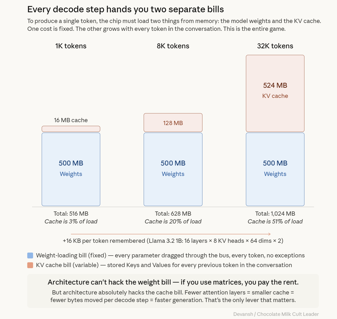
Transformers don’t just store weights; they store a growing memory of the conversation — the KV cache. Every new token adds to it, across every attention layer. For a small model like Llama 3.2 1B, that cache alone reaches ~524 MB at a 32K context. In practice, a single long interaction pushes total memory past a gigabyte. The bottleneck isn’t raw compute.
It’s memory that grows every time the model is used.
The transformer was designed for data centers where memory is abundant, and billing is per-token. On a phone, it is a structural mismatch. The architecture treats memory as infinite. The device does not.
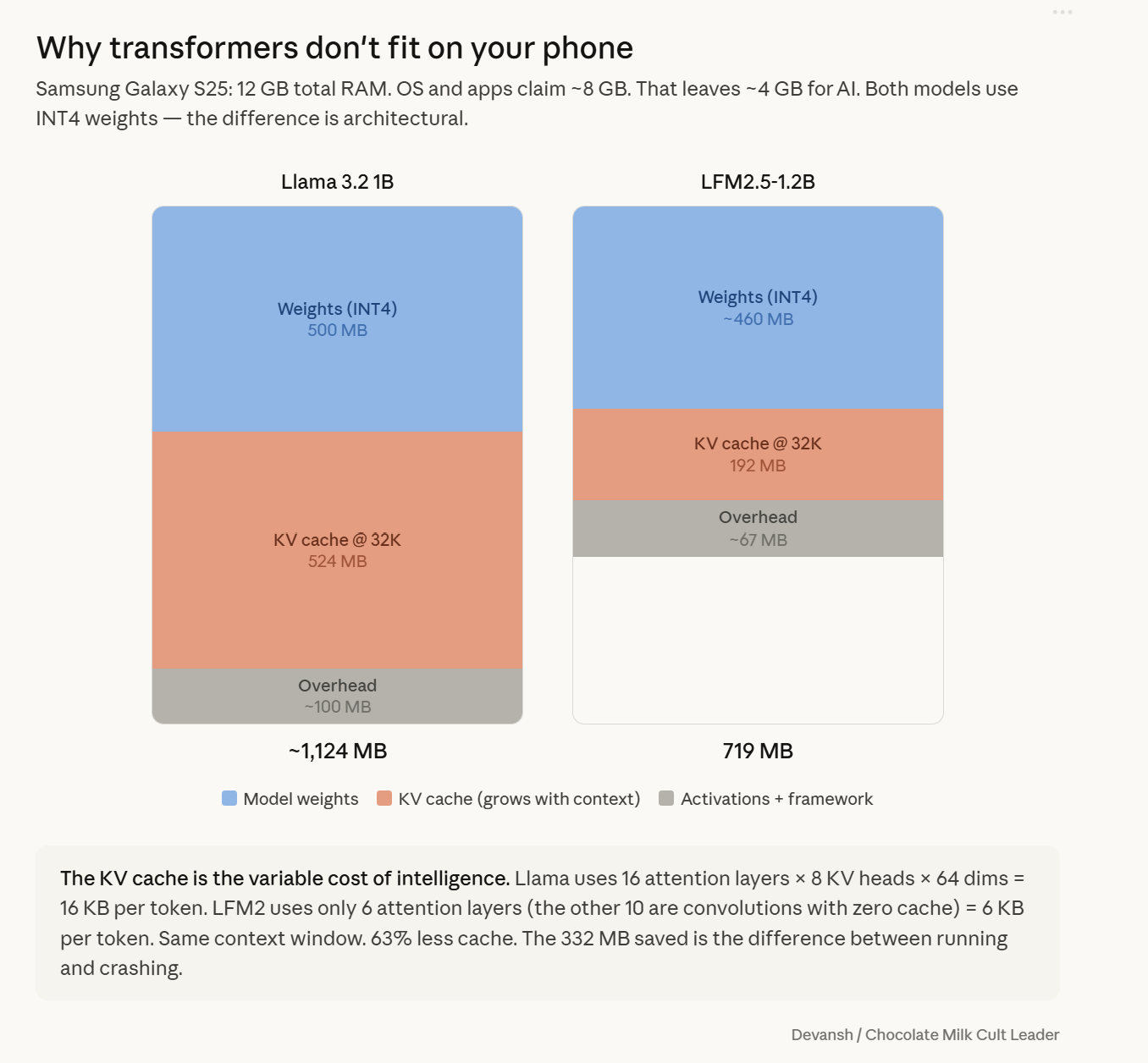
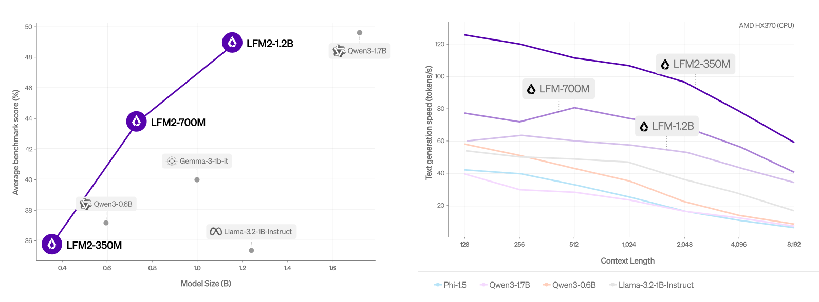
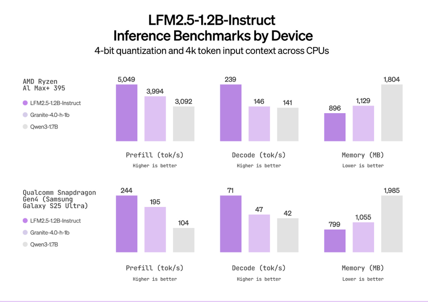
Liquid AI’s LFM2 changes this. Their 1.2-billion-parameter model runs on that same Galaxy S25, full 32,000-token context, in 719 megabytes total. Seventy tokens per second on the CPU on the same quantization scheme as above. It is a fundamentally different answer to the question of which operations should persist in memory and which should not.
In this article, we will walk through how Liquid AI built the best edge model in the world, from scratch. By the end, you will understand the following:
Why transformers become expensive on edge devices (memory, bandwidth, KV cache growth)
What alternatives exist, and what they give up (SSMs, linear attention, hybrids)
How Liquid AI’s architecture works and why it’s different from the status quo.
Why their search system (STAR) may matter more than the model itself
What the benchmarks and real-device performance actually show
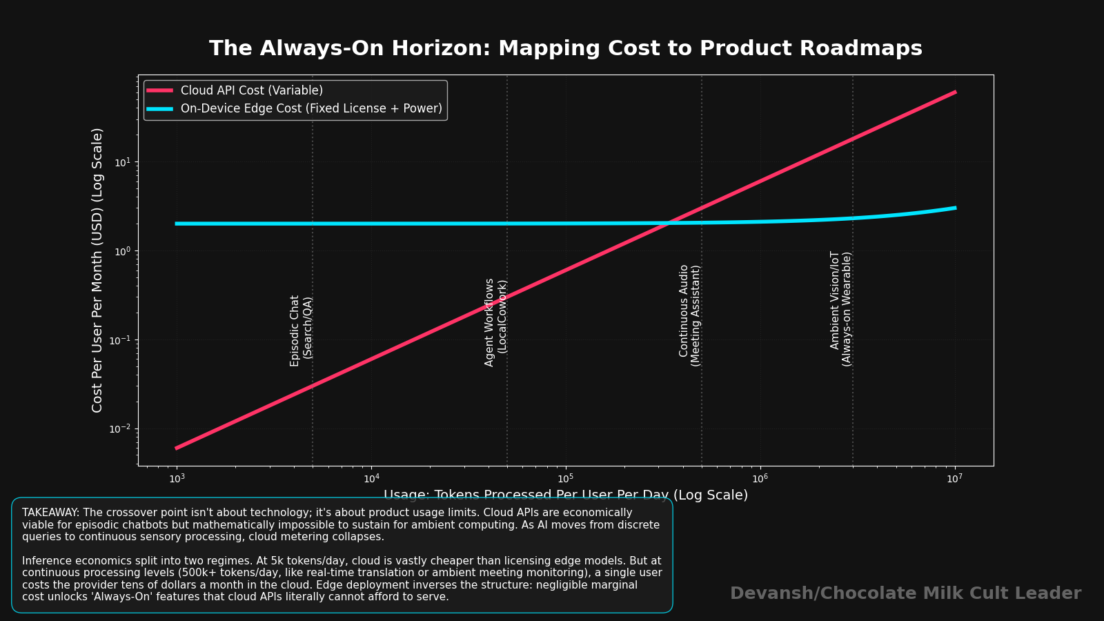
Where the economics flip from cloud to on-device
What could break this entire thesis
As with our other deep dives, you won’t need any prior knowledge. I will walk you through everything you need to know, ground up. The goal is not just to explain how one strong edge model works, but to show where low-cost, high-efficiency AI is heading next.
Executive Highlights (tl;dr of the article)
The bottleneck on your phone is memory bandwidth, not compute. Single-token decode has an arithmetic intensity of ~4 FLOPs/byte on hardware built for 295. Your H100 runs at 1.4% utilization. Your phone is 49x worse on bandwidth and can’t batch. The KV cache grows 16 KB per token for Llama 3.2 1B — 524 MB at 32K context, larger than the model weights. Quantization halves the per-token cost but doesn’t stop the growth.
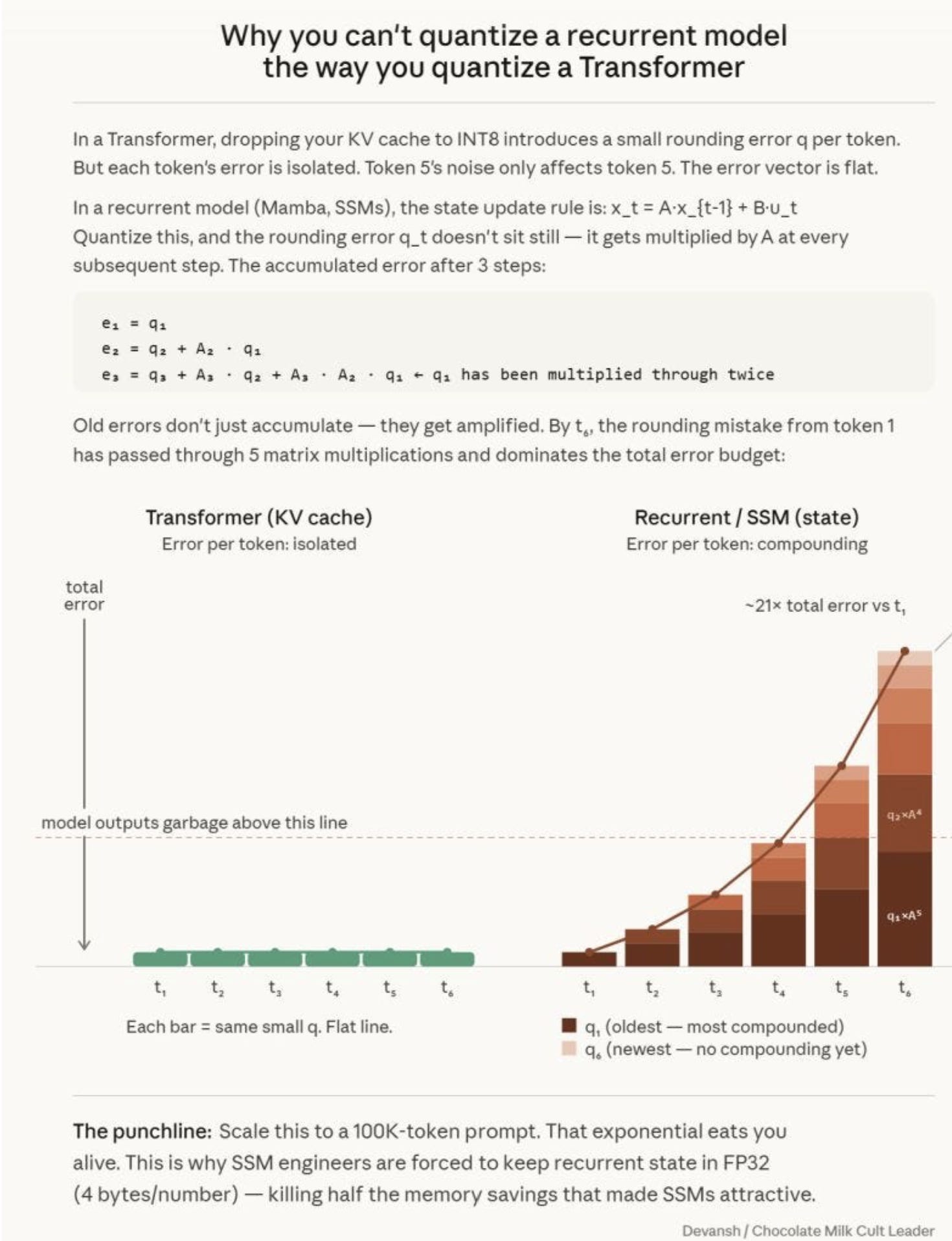
Every alternative architecture sacrifices something. SSMs: O(1) memory but compound quantization errors multiplicatively (fatal on INT4 edge hardware). Linear attention: kills quadratic math but token associations bleed together. Convolutions: fast, 15 years of mobile optimization, but blind past their window. No single mechanism works alone.
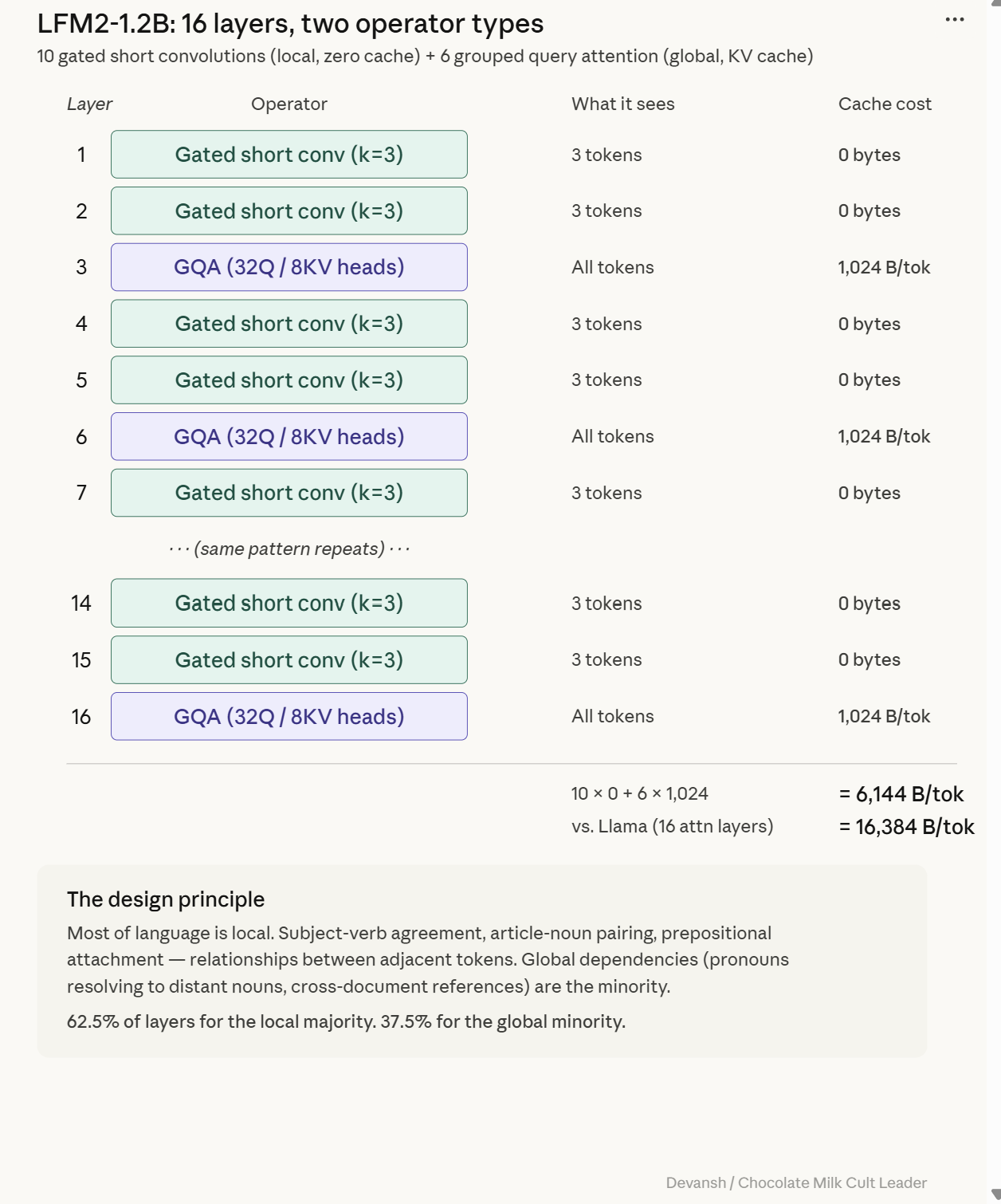
LFM2: 10 gated short convolution blocks + 6 grouped-query attention blocks. Convolutions handle local syntax with zero cache. Attention handles global retrieval, deployed sparingly. 192 MB cache at 32K vs. Llama’s 524 MB — 63% cut from fewer attention layers, 90% reduction with grouped-query sharing.
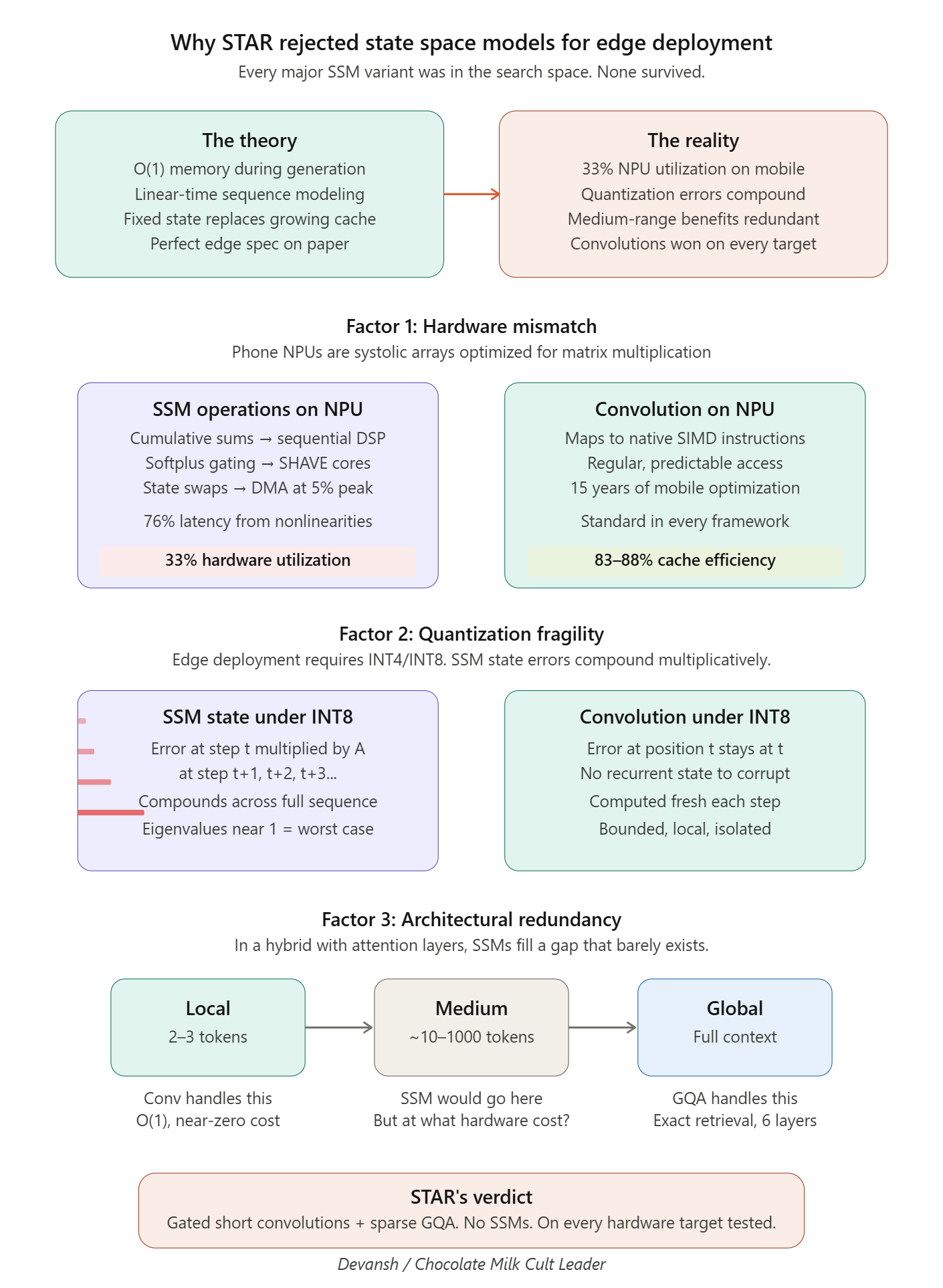
STAR matters more than the model. An evolutionary search system that encodes architectures as hierarchical genomes and evolves them on actual phones under real latency/memory constraints. The key upgrade: replaced proxy metrics with hardware-in-the-loop profiling on Galaxy S24s and Ryzen laptops. Proxy metrics lie — Mamba and convolutions have similar theoretical FLOPs but convolutions map to native SIMD instructions. STAR rejected every SSM variant.
The training pipeline closes the gap against models 42% larger. Distillation from a 7B teacher storing only top-32 logits (2,000x compression) with a decomposed loss that separates membership from ranking. Curriculum learning easy-to-hard. Model merging at zero inference cost. INT4 quantization in the loop from the start.
Three unsolved problems determine who wins edge AI. Signal-to-noise (ambient computing means 99% of tokens are garbage — architectures must actively refuse to process context). Hardware fragmentation (no standard edge chip — either vertical players capture the edge or open-source builds a communal STAR). Hostile markets (healthcare, defense, industrial — 700 MB of local intelligence bypasses the cloud entirely).
I put a lot of work into writing this newsletter. To do so, I rely on you for support. If a few more people choose to become paid subscribers, the Chocolate Milk Cult can continue to provide high-quality and accessible education and opportunities to anyone who needs it. If you think this mission is worth contributing to, please consider a premium subscription. You can do so for less than the cost of a Netflix Subscription (pay what you want here).
I provide various consulting and advisory services. If you‘d like to explore how we can work together, reach out to me through any of my socials over here or reply to this email.
1) The Main Hardware Constraint for AI Inference: Memory Bandwidth
Most people assume the hard part of running an AI model is the math. Bigger brain, more parameters, heavier multiplications, beefier chip. It’s a beautifully clean, totally intuitive mental model — and just like most other thoughts you have in your life, it is in a passionate “no-contact” with intelligence or reality.
The binding constraint on modern inference — especially on phones, laptops, and edge devices sweating in your pocket — isn’t how fast the chip can do math. It’s how fast the chip can feed itself data to do the math. Erling Haaland with a Spursy midfield wouldn’t get any goals.
How Language Models Generate Text: Prefill vs. Decode
A language model spits out text one token at a time. Generation is autoregressive, which is just a fancy way of saying it’s inherently serial: step 1, then step 2, no skipping ahead. But this process has a split personality.
Phase 1: Prefill. This is the honeymoon phase. The model receives your entire input prompt at once, and because those tokens already exist, it can process them all in parallel. Prefill is a massive, compute-heavy rave. Everyone is dancing, the hardware is maxed out, and the chip gets to flex its muscles.
Phase 2: Decode. The hangover. This is where the economics get brutal. The model now has to generate tokens one by one. Every single token requires a full pass through every layer of the model. But because you are only producing one word, your “batch size” is exactly 1. You are multiplying the model’s entire weight matrix against a single tiny vector just to produce one number. Then you do it gain. And again.
Decode doesn’t stop being a problem here. This diva also comes in with 2 different cost profiles that you need to worry about.
The Two Memory Costs: Weight-Loading and Cache-Access
Every decode step hands you two separate bills (reminds me of my dates):
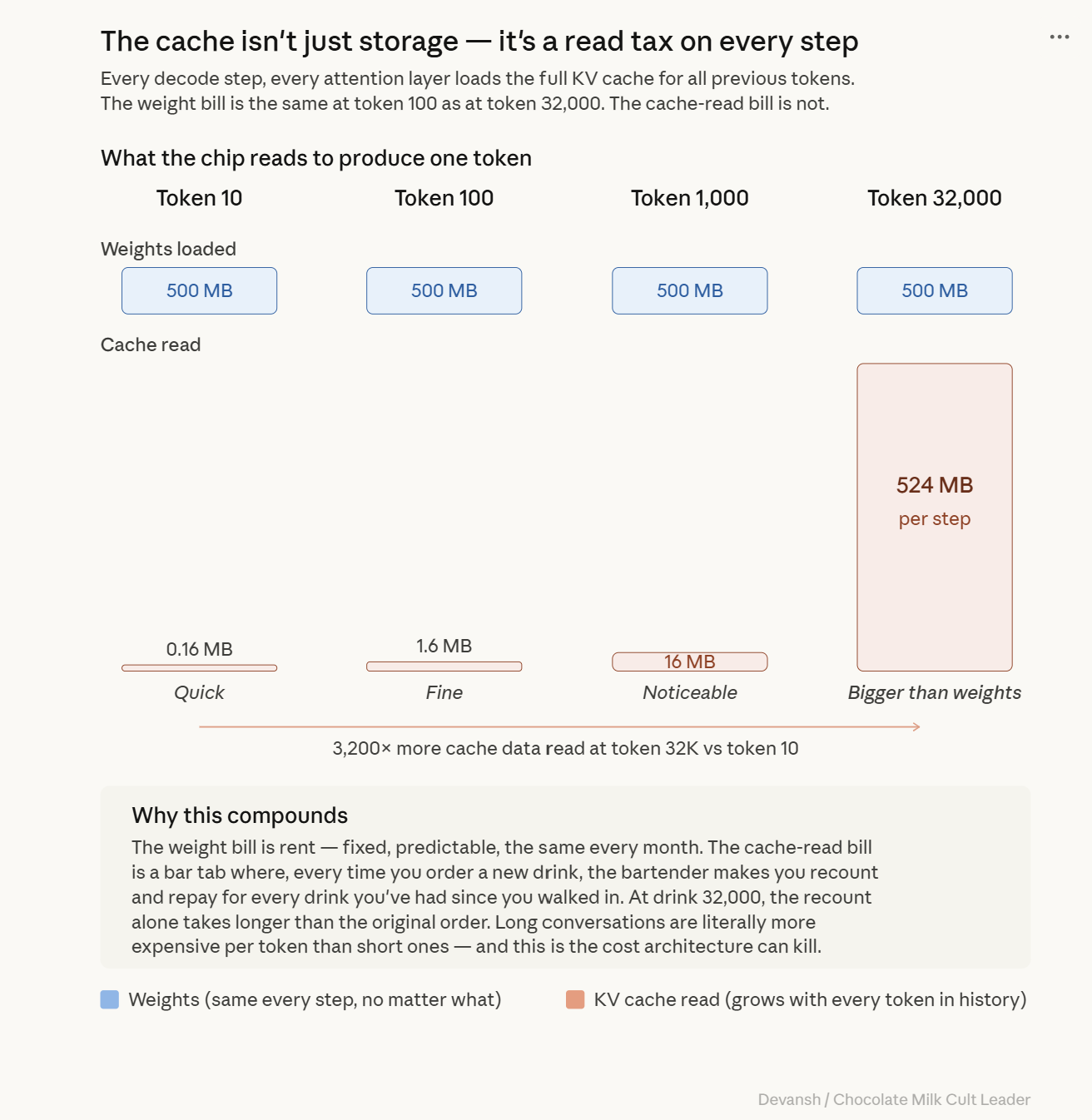
The Weight-Loading Bill (Fixed): To produce a single token, every parameter in the model must be dragged from memory into the processor. For a 1B model at INT4, that is roughly 500 megabytes shoved through the memory bus. Per token. Every fucking token. The model doesn’t get to skip layers because the answer is an easy word like “the.” The full weight matrix moves, every time.
The Cache-Access Bill (Variable): The model must also read the KV cache (the stored memory of previous tokens) to compute attention. At token 100, this cache is cute and small. At token 32,000, it’s a bloated monster that might literally be larger than the weights themselves. If the weight-loading bill is your rent, the cache-access bill is a taxi meter in Manhattan traffic while the oil and gas industry uses every world event to price-gouge profits from you.
That is why the key metric here is not FLOPs in isolation, but arithmetic intensity: how much useful computation the chip gets for every byte it has to move. Let’s look at how.
Arithmetic Intensity Explained: FLOPs Per Byte
If you want to understand why a chip with massive theoretical compute can still deliver painfully slow inference, you need to know one number: Arithmetic Intensity.
It’s the ratio of useful math to data dragged around. FLOPs per byte. For every byte the chip pulls from memory, how many multiplications does it get to do before it starves for the next one?
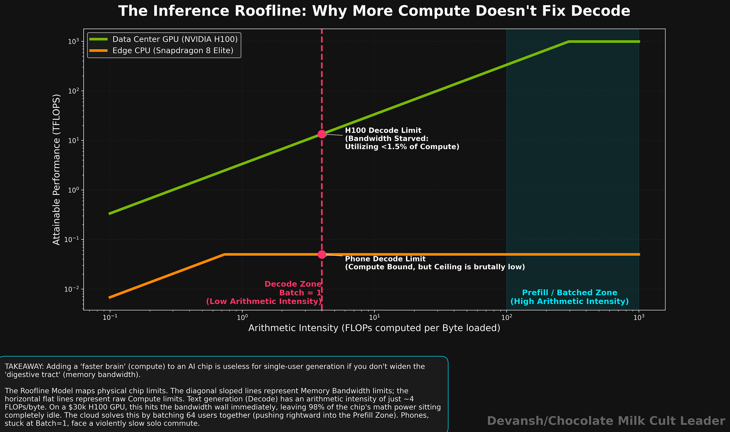
During decode, a single token is multiplied against each weight exactly once. For a weight stored in INT4 (0.5 bytes), your arithmetic intensity is roughly 4 FLOPs per byte. That ratio holds no matter how big your model is. It’s a property of the operation, not the chip.
Now, look at the hardware. An NVIDIA H100 — the $30,000 GPU currently holding the global economy hostage — has a compute-to-bandwidth ratio of roughly 295 FLOPs per byte. But your decode phase only needs 4. During single-user text generation, your H100 is running at a pathetic 1.4% of its theoretical peak. Erling Haaland in the opposition box, waiting for the balls that will never come.
Understanding this failure in more detail requires us to look at the Roofline Model. The roofline model asks a simple question: for a given operation, which limit does the chip hit first?
The Roofline Model: Compute Limits vs. Bandwidth Limits
Every chip has two hard limits:
A Compute Ceiling: Max operations per second (the brawn).
A Bandwidth Ceiling: Max bytes per second from memory (the digestive tract).
Whichever ceiling you hit first is your bottleneck. Single-token decode at 4 FLOPs per byte smacks its head against the bandwidth ceiling on virtually every data center GPU in existence. The chip has compute to spare and nothing to feed it.
This is why tossing a “faster chip” at inference doesn’t work. A chip with 2x more compute but the same memory bandwidth will generate tokens at the exact same speed, because the bottleneck was never the math. The only way to go faster is to move fewer bytes per token, or build wider pipes.
And all of that leads to our original question — why is it so hard to get on-device generative AI right?
Why Inference is Slower on Edge Devices vs. Data Centers
Data centers survive this bottleneck because they have three cheat codes phones don’t: deep memory, massive bandwidth, and batching.
When 64 users hit an H100 at the same time, the GPU loads the weights once and applies them to all 64 tasks. The cost per user drops by 64x. Batching is the holy grail of cloud economics (that’s why API providers offer discounts on it). But a phone? A phone is a sad solo commute. Batch size is 1. There is nobody to split the bill with.
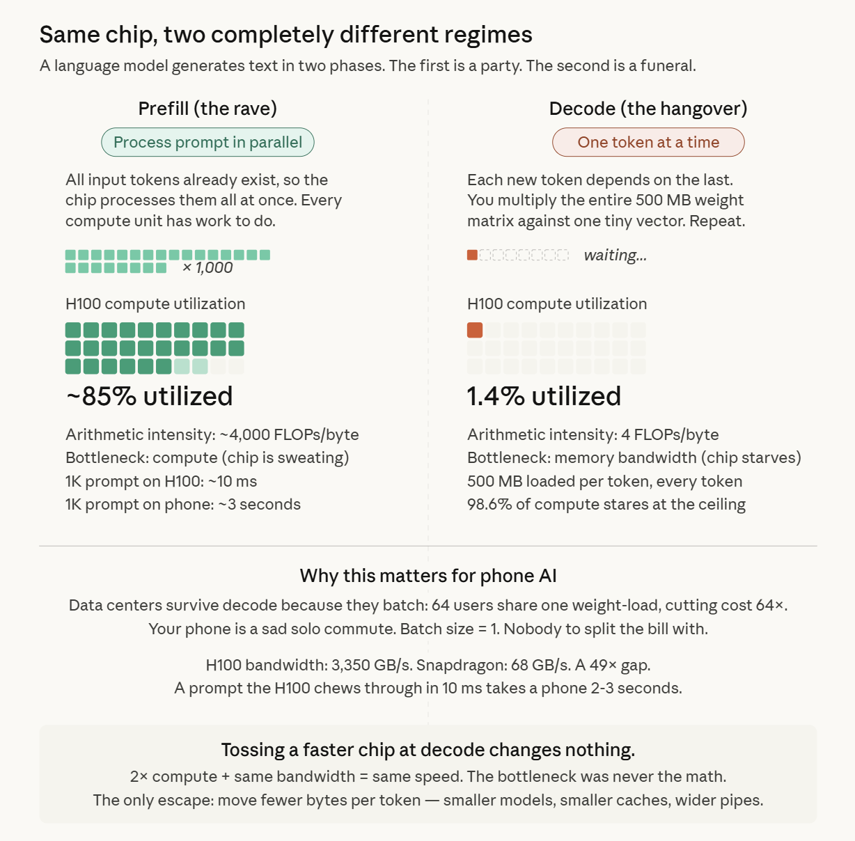
Then there’s the bandwidth gap. An H100 delivers roughly 3,350 GB/s. Your flagship Snapdragon? Maybe 77 GB/s. That is a 49x gap. Weights that take an H100 a breezy 0.15 milliseconds to load take your phone 7 milliseconds. Per token. A prompt the cloud chews through in 10 milliseconds takes a phone CPU 2–3 excruciating seconds. You know that awkward pause before your AI assistant starts talking? That’s your phone violently shoving data through a tiny pipe.
Oh, and the H100 has 80 gigabytes of dedicated high-speed RAM. Your phone has 12 gigabytes of shared RAM, and half of it is already being hogged by your browser tabs.
Architecture cannot outrun the weight-loading bill — if you use matrices, you pay the rent. But architecture can absolutely hack the cache-access bill. Fewer attention layers equals a smaller KV cache. A smaller cache means fewer bytes read per decode step. Fewer bytes means you avoid that nasty bandwidth ceiling.
The real question isn’t “how do we make transformers faster on phones?” The question is: “which of these operations actually deserve to take up precious memory, and which ones are just burning our battery for absolutely no reason?”
And with that super slick transition, it’s time for us to take a deep look at the drivers of cost, and what we can drop.
2) The Transformer’s Memory Cost Structure: Weights vs. KV Cache
We already established that the decode phase hands you two memory bills. One is a predictable baseline; the other is a compounding tax. Let’s look at the receipt.
The Fixed Cost: Model Weights
Model weights are your fixed cost. For a 1B model at INT4, you are moving roughly 500 MB through the memory bus per token. You load it, apply it layer by layer, and move on. The size of the model does not change whether your prompt is three words or 20,000. It is a strictly known quantity, which makes it a manageable engineering problem.
Unfortunately, the transformer brought a parasitic plus-one.
The Variable Cost: The KV Cache
In every attention layer, for every single token processed, the transformer stores two vectors: a Key and a Value. This stored history is the KV cache. Unlike the weights, it grows with every token generated.
The growth rate is mathematically rigid, baked into the architecture at design time:
Cache per token = 2 * attention layers * KV head groups * dimension per head * bytes per element
Every variable there except sequence length was chosen by the architect long before training started. The hardware just eats whatever they chose. Look at Llama 3.2 1B. Every token adds exactly 16,384 bytes. About 16 KB per token. Sounds harmless. Watch context scale:
At 4,000 tokens (short conversation): 65 MB.
At 32,000 tokens (real conversation): 524 MB. The cache is now larger than the weights.
At 128,000 tokens (where every product roadmap points): 2 GB. Game over on a phone.
Saying “the cache grows linearly” is technically correct and entirely useless. “Linear growth” can mean manageable overhead, or it can mean your phone violently murders background apps just to keep breathing.
And finding the RAM for that bloated cache isn’t even the worst part. You also have to keep reading it.
The Decode Memory Tax: Reading the KV Cache
The KV cache is highly active memory traffic. Every decode step, every attention layer loads the full cache for all previous tokens to compute attention scores. At token 100, you read 100 cached pairs per layer. Quick. At token 32,000, you read 32,000 pairs per layer — a 320x increase in data movement.
The weight-loading bill is the exact same at token 100 as it is at token 32,000. But the cache-access bill keeps climbing. Long conversations are literally more expensive per token than short ones. And just when memory bandwidth is tapped out, the attention math swoops in to make things exponentially worse.
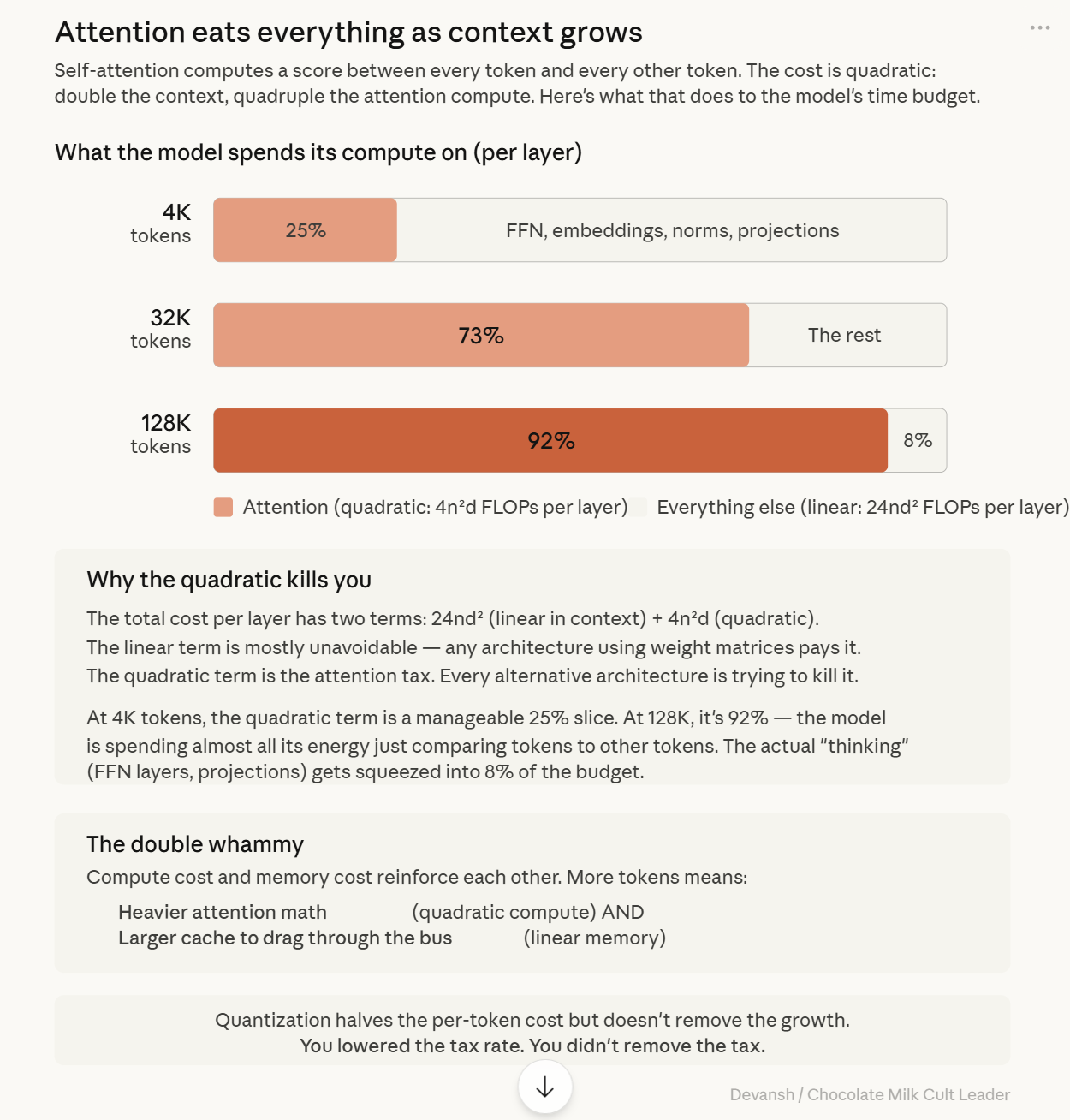
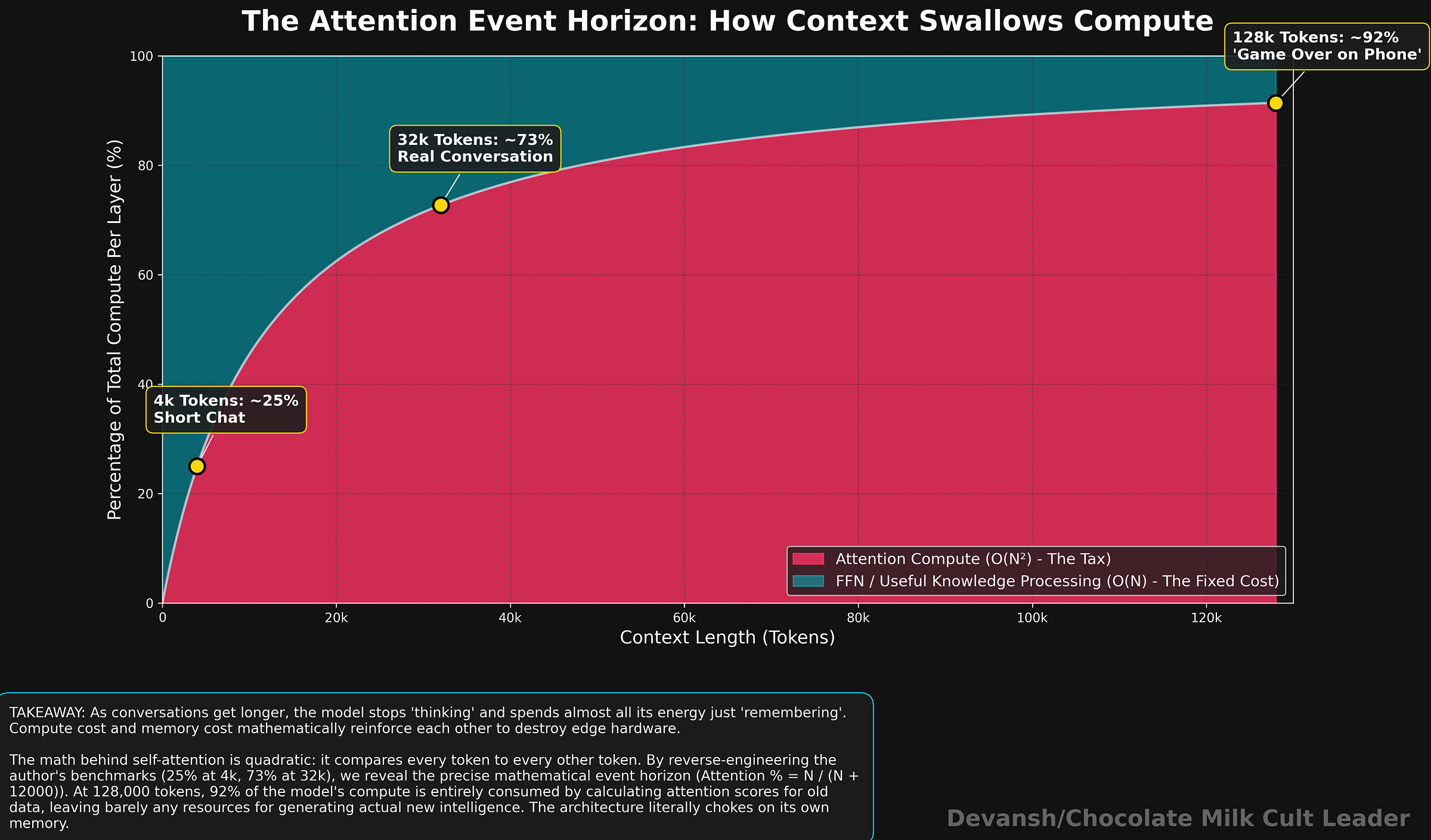
Why Self-Attention Compute Costs Grow Quadratically
Standard self-attention computes a score between every token and every other token. The compute cost is quadratic, swallowing your budget as context grows:
At 4,000 tokens: Quadratic attention is roughly 25% of total compute per layer.
At 32,000 tokens: ~73%. Attention is now the vast majority of what the model does.
At 128,000 tokens: ~92%. The model spends almost all its energy just looking at things it already looked at.
Compute cost and memory cost reinforce each other. More tokens means heavier attention math AND a larger cache to drag through the bus. Both hardware ceilings drop simultaneously. This is why long-context inference attacks both constraints at once. So, if the cache is bloated and the math is heavy, can’t we just compress the numbers and call it a day?
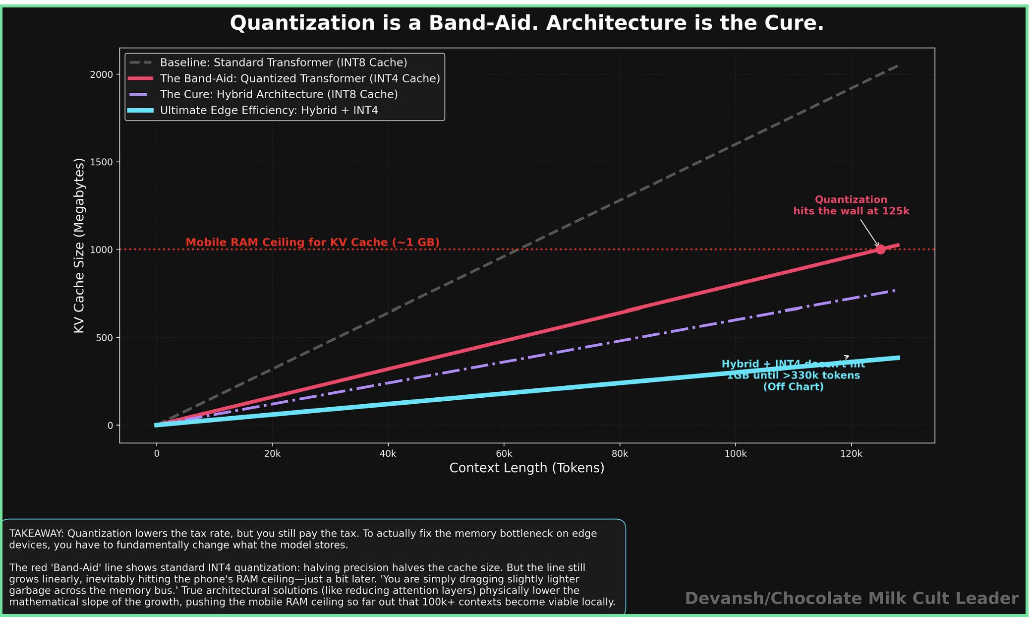
Why Quantization Does Not Solve the Memory Bottleneck
Quantization is compression, not absolution. Halve the precision, you halve the per-token cost. Great. But the cache still grows linearly. The model still reads that entire cache every decode step. You lowered the tax rate; you didn’t remove the tax. You are simply dragging slightly lighter garbage across the memory bus, and that bus will still max out.
Also, aggressive quantization hurts small models far more than large ones. Squeezing a 1B model to INT4 hits it disproportionately hard. This is why Liquid AI trains with quantization in the loop from the start — learning to be good despite the rounding, rather than getting brain damage later.
So, where does this technical butchery leave us for shipping products?
The Real Question: What Happens After the Twentieth Reply?
Model weights are the fixed cost you pay because the model exists. The KV cache is the variable cost you pay because the conversation exists. You are not charged extra because the model got bigger; you are charged extra because the interaction got longer.
Edge devices are uniquely allergic to variable costs because their memory budget is a joke and their bandwidth pipe is a straw. The question stops being “can I cram this model onto the device?” and becomes “what happens to this device after the twentieth reply?”
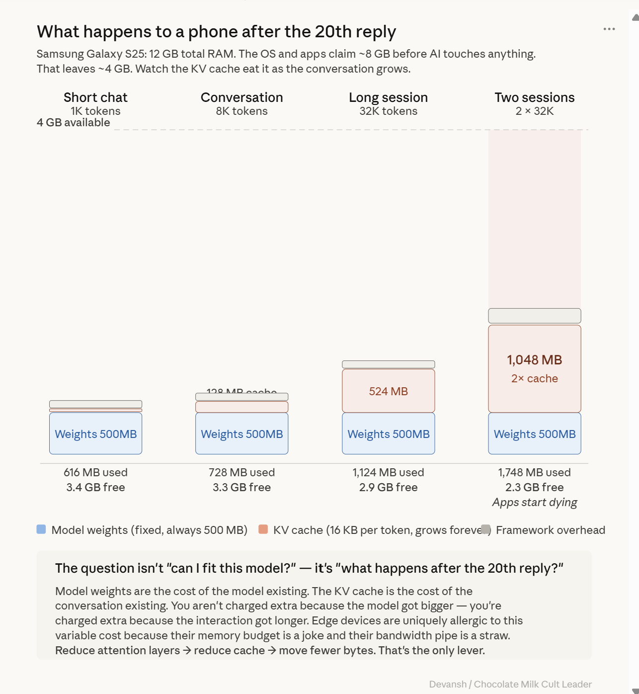
If we can’t escape the fixed weight-loading bill, our biggest lever is the variable cache-access bill. Reduce attention layers. Reduce explicitly preserved history. Move fewer bytes. This is where architecture becomes raw deployment economics.
Every alternative architecture is just trying to kill some part of this bill while giving something else up. Some compress the cache, some use fixed state, some use convolutions.
So now that we know exactly how the transformer is extorting us, what are the escape routes, and what does each alternative sacrifice?
3) The Escape Routes: Alternatives to Standard Attention
We’re keeping this section deliberately light since we have a massive deep dive into the first 3 of these alternatives in one place over here: “How Long Context Inference Is Rewriting the Future of Transformers”. The 4th — convolutions — will be broken down here since it’s the crux of Liquid AIs push.
Every alternative AI architecture proposed in the last five years is trying to solve the exact extortion racket we just outlined. They look at the transformer’s variable KV cache tax and the quadratic attention compute, and they desperately look for a fire exit.
But physics is ruthless. You cannot get full global attention for free. Every single escape route forces a sacrifice. The entire architectural design space is just a hostage negotiation over what you are willing to lose to lower your memory and compute bills.
Let’s walk through the four desperate attempts the field has made to dodge the check.
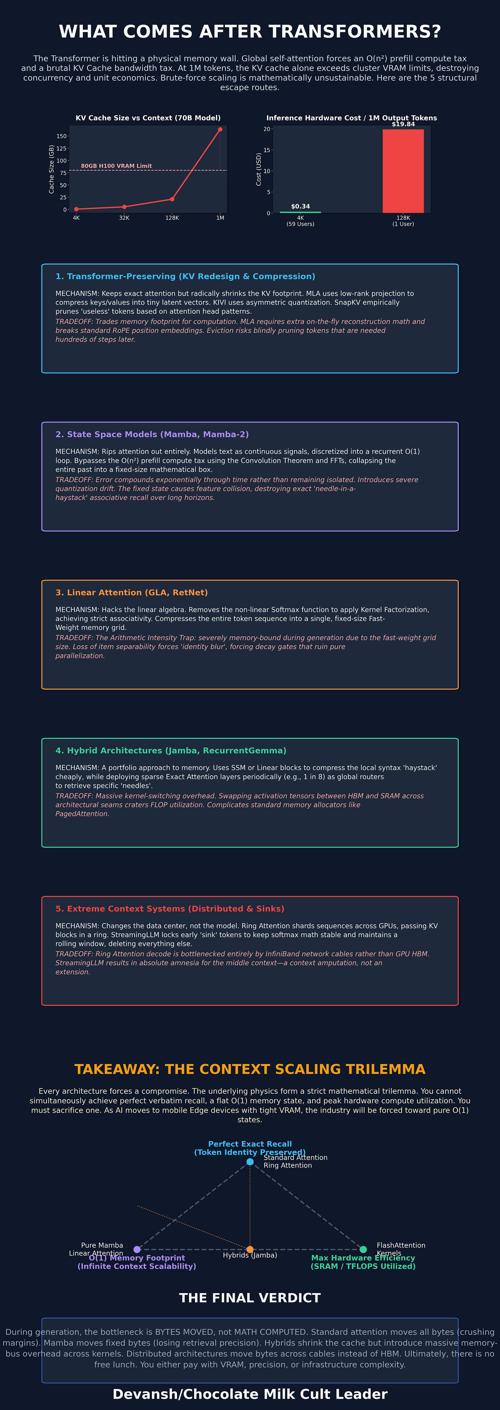
Escape Route 1: Compressing the KV Cache
If the KV cache is too big, the most obvious engineering solution is to simply store less of it. You keep the transformer architecture exactly as it is, but you aggressively compress the receipt.
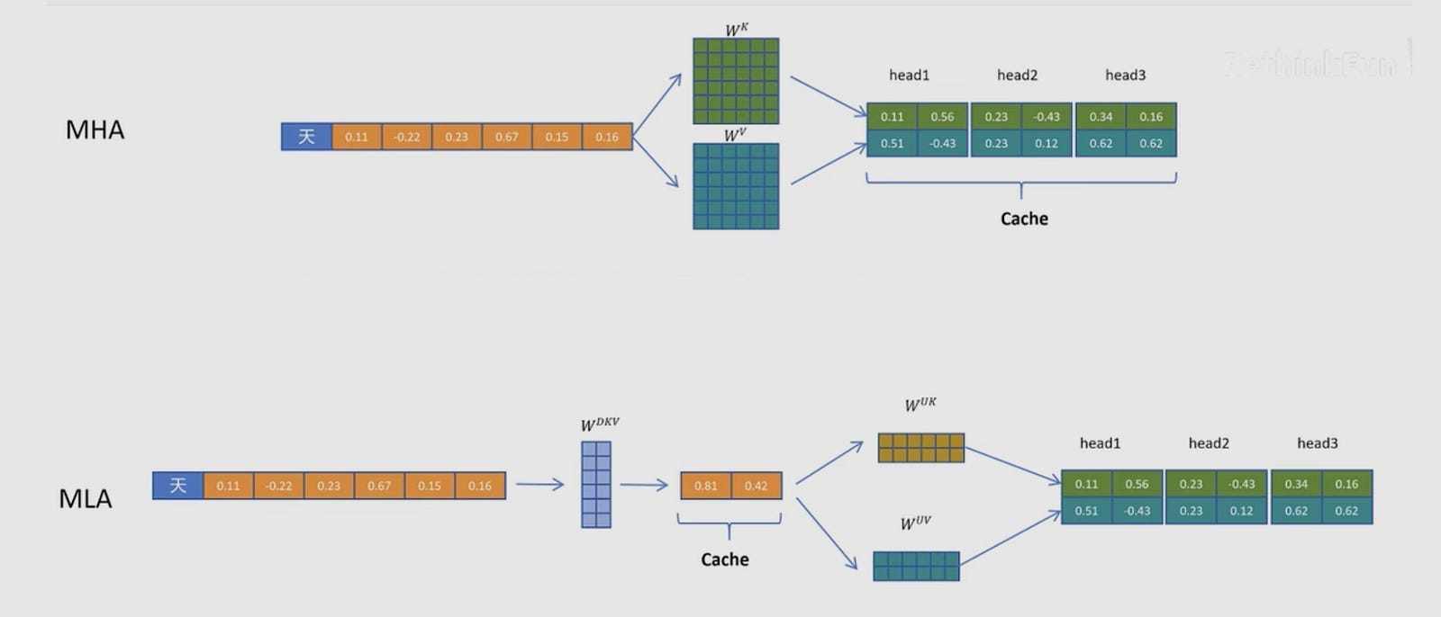
Multi-head Latent Attention (DeepSeek): Projects the Key and Value vectors into a tiny compressed representation before storing them, reinflating them on the fly when needed.
SnapKV: Looks at the tokens and literally just throws away the ones the attention heads rarely look at, much like a cat making direct eye contact with you while slowly swatting your keys off a table because they aren’t relevant to its immediate needs.
PagedAttention (vLLM): Doesn’t shrink the cache, but stops it from fragmenting your RAM by storing it in non-contiguous blocks, like virtual memory on a PC.
What it buys you: You can slash the size of the cache by 60% to 90%.
What it costs you: The growth rate shrinks, but the growth does not stop. Even if you compress the cache by 90%, an ambient agent listening to 100,000 tokens a day will eventually consume your phone. Compression delays the memory wall; it does not remove it.
Delaying the memory wall isn’t a long-term strategy. If you actually want to stop the bleeding, you have to burn the cache entirely.
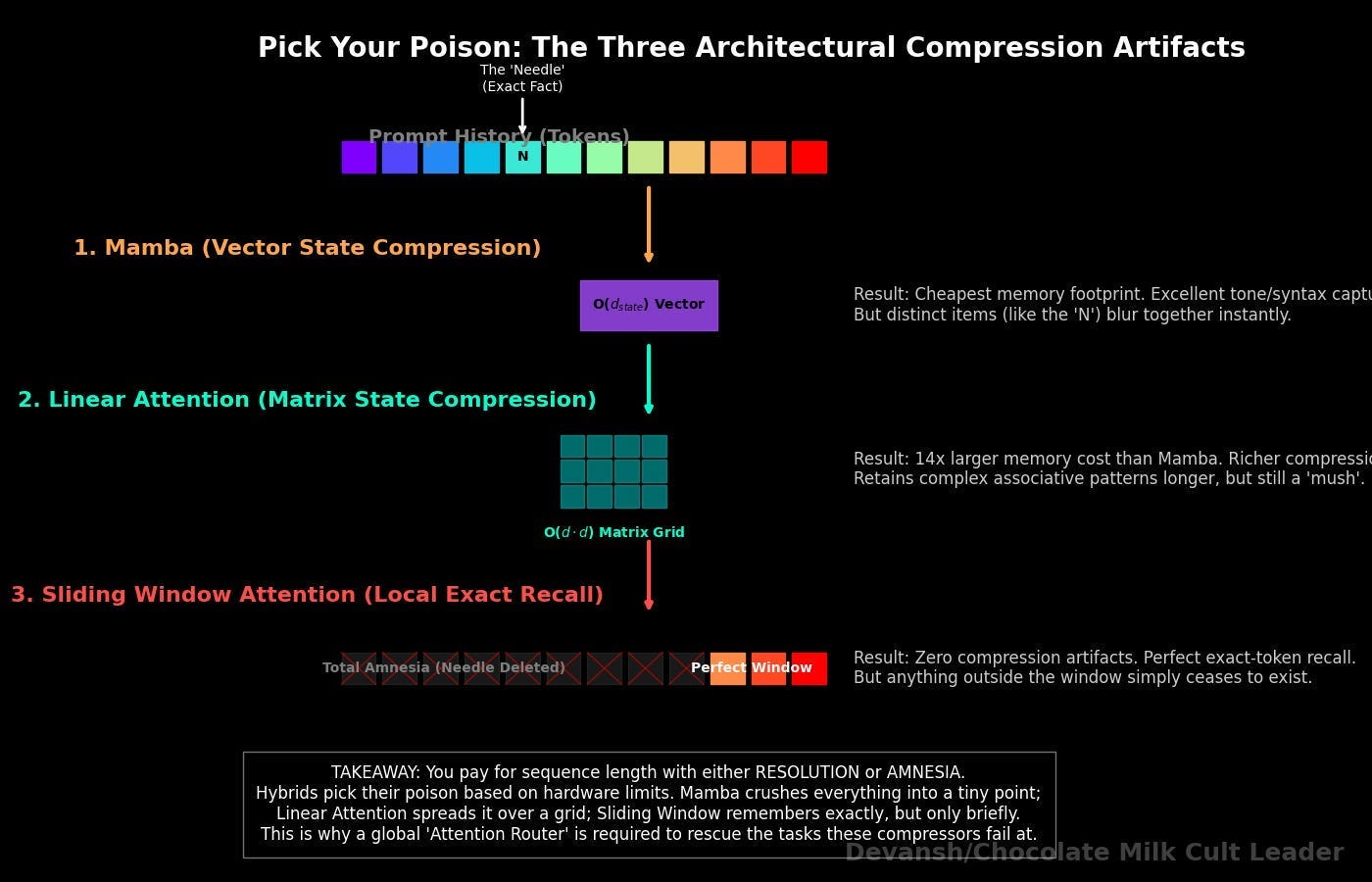
Escape Route 2: State Space Models (SSMs) and Mamba
If you refuse to let the memory footprint grow, you have to abandon the KV cache. Enter State Space Models (SSMs).
Instead of storing a perfect record of every token you’ve ever seen, an SSM compresses the entire history of the conversation into a single, fixed-size mathematical box (a state vector). When a new token arrives, the model updates the state vector, and then throws the raw token in the trash.
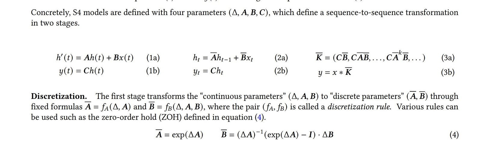
What it buys you: O(1) memory during generation. Your memory footprint is exactly the same at token 10 as it is at token 100,000. It is theoretically the perfect edge architecture.
What it costs you: Precision. Because the state is a fixed size, it is a lossy compressor. It remembers the general vibe and the narrative, but over long sequences, individual token identities blur together — exactly like trying to recall the specific sequence of a combo after taking a clean right hook to the jaw during a sparring session. You know what happened, but the granular details are gone. If you ask an SSM to retrieve a highly specific, verbatim quote from token 5 in a 100,000-token document, it will hallucinate or fail where a transformer would succeed effortlessly.
If memory loss isn’t an acceptable trade-off for your product, you have to try cheating the math instead of the storage.
Escape Route 3: Linear Attention
Standard attention compares every token to every other token, creating that enormous, sequence-length-dependent n-by-n matrix. Linear attention uses a clever algebraic trick to change the order of operations. It applies a feature map and multiplies the matrices in a different order, creating a fixed-size d-by-d matrix that does not grow with the sequence length.
What it buys you: Like SSMs, memory during generation becomes fixed. You completely kill the quadratic compute cost.
What it costs you: Feature collision. Linear attention mashes all the token associations additively into a single matrix. Over a long conversation, these features overlap and bleed into each other. It’s the mathematical equivalent of shoving your clean everyday clothes, sweaty MMA rash guards, and loose climbing chalk into the exact same duffel bag. Everything is technically in there, but good luck pulling out a clean shirt without it smelling like a bouldering gym.
If global math gets too messy, the only remaining option is to stop looking at the big picture entirely.
Escape Route 4: Long Convolutions
Before transformers took over, researchers processed sequences using convolutions. A convolution slides a mathematical window over the text, mixing information locally. It doesn’t look at the whole document at once; it just looks at the tokens immediately around it.
What it buys you: Hardware absolutely loves convolutions. Mobile CPUs have been optimizing convolutional math for image processing for 15 years. They are blazingly fast and require virtually no memory overhead.
What it costs you: Blindness. If you use a convolution, you only see what is inside your window. If a pronoun needs to resolve to a noun 5,000 tokens ago, a convolution literally cannot see it.
When you look at the wreckage of this design space, a brutal reality emerges.
The Real Lesson: Hybrid Architectures Are the Only Way
Transformers give you perfect retrieval but bankrupt your memory. SSMs and Linear Attention fix your memory but blur your retrieval. Convolutions are incredibly fast but functionally myopic.
The field spent years arguing about which of these was the “right” answer. The actual lesson is that they are all the wrong answer if you apply them to the entire model.
If you want to build an architecture that survives on a phone, you cannot force one mathematical mechanism to do everything. You have to build a portfolio. You use cheap, fast, local operators for the vast majority of the work, and you strictly reserve the expensive, memory-hogging exact retrieval for the few layers that actually need it.
This is the exact hybrid insight that Liquid AI used to build LFM2. But to understand why Liquid AI arrived at their specific ratio of cheap-to-expensive layers, we need to look at where this company actually came from. Because they didn’t start by trying to fix the transformer. They started by trying to simulate the brain of a worm.
They started by trying to simulate the brain of a worm.
4) The Historical Path to Liquid AI — From Worm Brains to Foundation Models
If you look at the pedigree of most major AI labs — OpenAI, Anthropic, Mistral — all share the same evolutionary lineage. They are descendants of the original 2017 Transformer paper. Their entire scientific worldview is built on figuring out how to make self-attention bigger, faster, or slightly less gluttonous. And if they’re gay, they likely did a lot of work on stabilizing and scaling Reinforcement Learning.
Liquid AI did not come from this lineage. They did not start by asking, “How do we make a transformer cheaper?”
They started by looking at a worm.
How 302 Neurons Beat Brute-Force Math
Caenorhabditis elegans is a one-millimeter roundworm. It has exactly 302 neurons, which Scientists have mapped completely.
If you look at modern deep learning, 302 neurons is nothing. It is a rounding error inside a single layer of an image classifier. Yet, with those 302 neurons, this worm can navigate toward food, avoid toxins, respond to temperature changes, and mate. It executes complex, continuous survival behaviors without a massive parameter count.
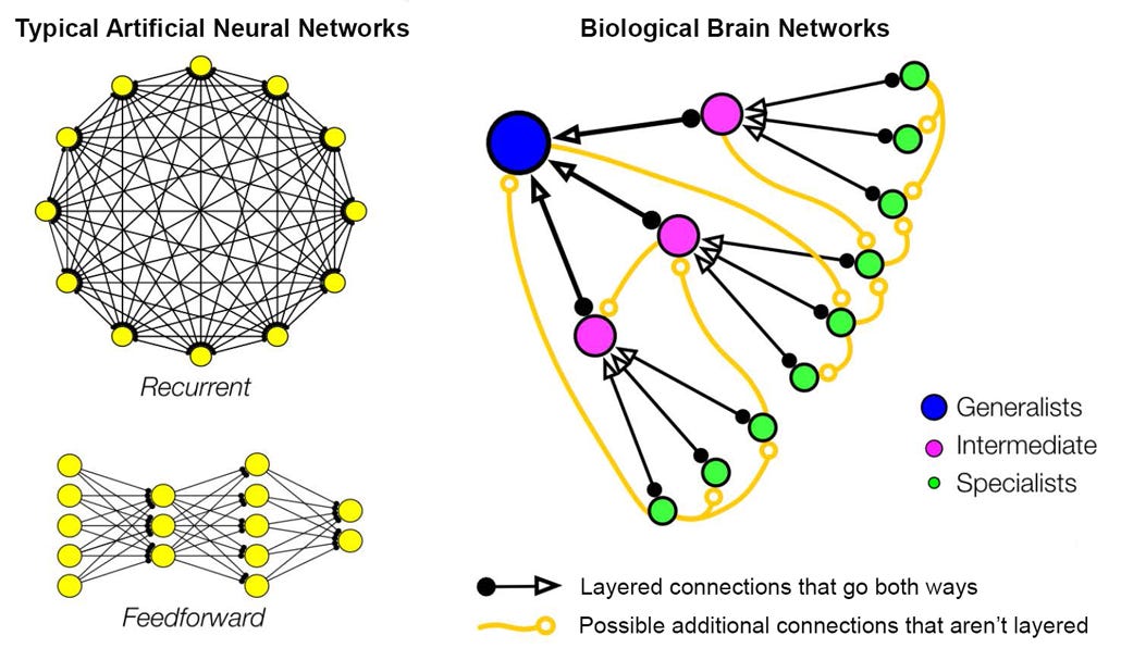
How does it pull this off? It cheats the math.
In a standard artificial neural network, the “weights” (the strength of the connections between neurons) are frozen after training. The network’s internal dynamics never change. In the worm’s brain, the strength of a synaptic connection changes dynamically based on the signals currently flowing through it. The time it takes a neuron to respond to an input is not a fixed parameter; it adapts on the fly depending on what the worm is looking at.
The founding team of Liquid AI — Ramin Hasani, Mathias Lechner, Alexander Amini, and Daniela Rus (director of MIT’s CSAIL) — looked at this and asked a brutal question: What if artificial networks stopped relying entirely on brute-force scale, and started adapting their internal dynamics to the input, exactly like the worm?
Liquid Time-Constant Networks: The First Breakthrough
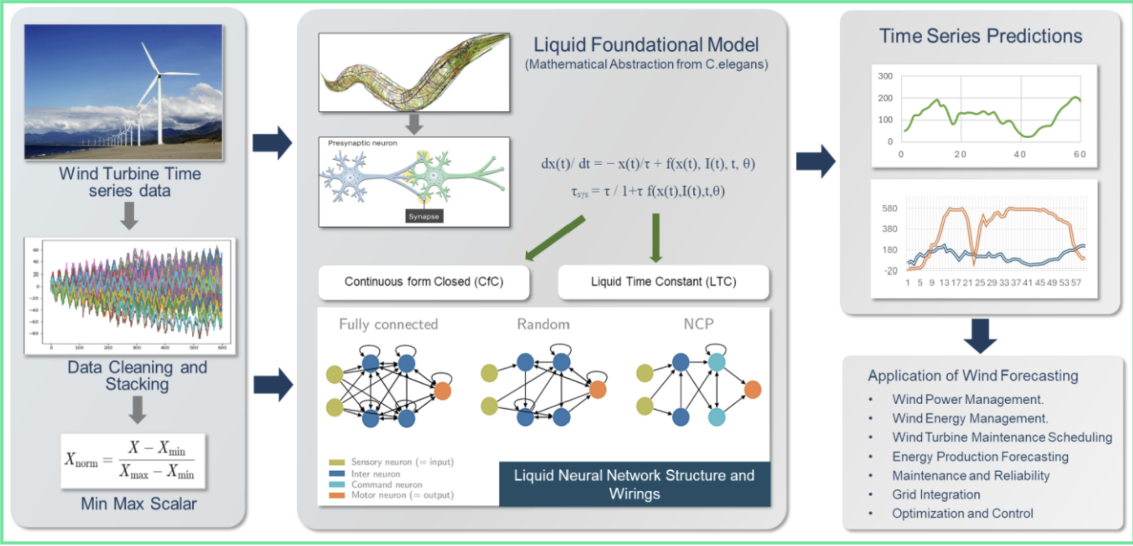
This obsession led to their first major paper in 2021: Liquid Time-Constant (LTC) Networks.
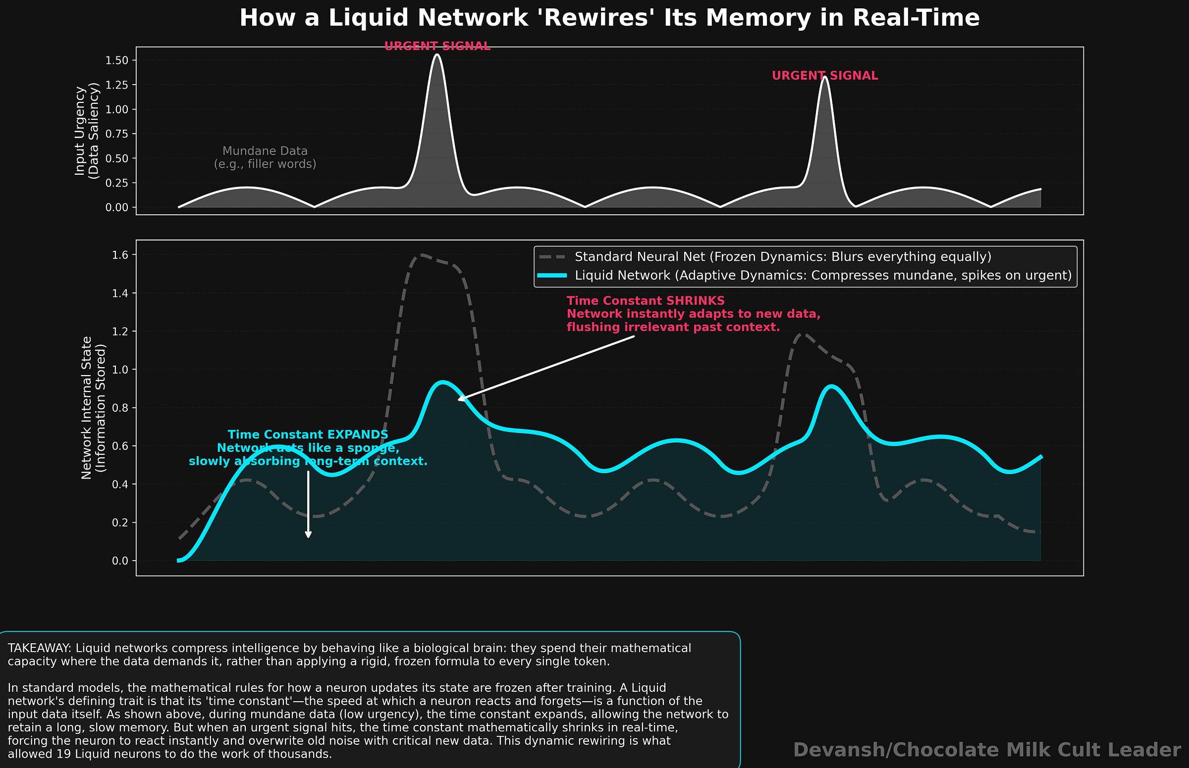
Instead of freezing the network’s behavior, they governed each artificial neuron with an ordinary differential equation (ODE). The “time constant” — the speed at which the neuron reacts and forgets information — was programmed to be a function of the input itself.
If a strong, urgent signal came in, the neuron’s time constant shrank, forcing it to react instantly. If a weak signal came in, the time constant expanded, allowing the neuron to slowly accumulate information and retain memory over longer periods. The network was literally rewiring its own temporal dynamics in real-time.
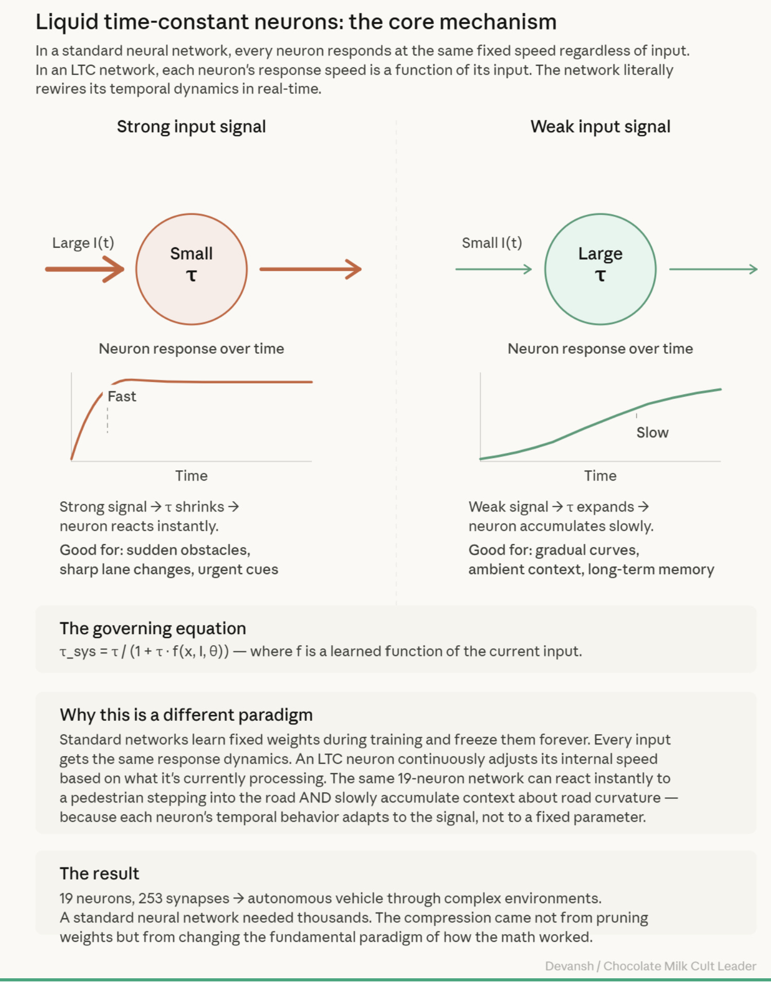
The result was staggering. They took a network with just 19 control neurons and 75K params to successfully drive an autonomous vehicle through complex visual environments. A standard neural network required thousands of neurons to do the same job. They also showed strong robustness in noisy scenarios.
But in software engineering, there is always a catch.
The Math Was Too Heavy
LTC networks were elegant, but computationally miserable to run.
Because they relied on ordinary differential equations, the computer had to use an iterative numerical solver for every single forward pass. Training was excruciatingly slow. Inference? Practically unusable at scale.
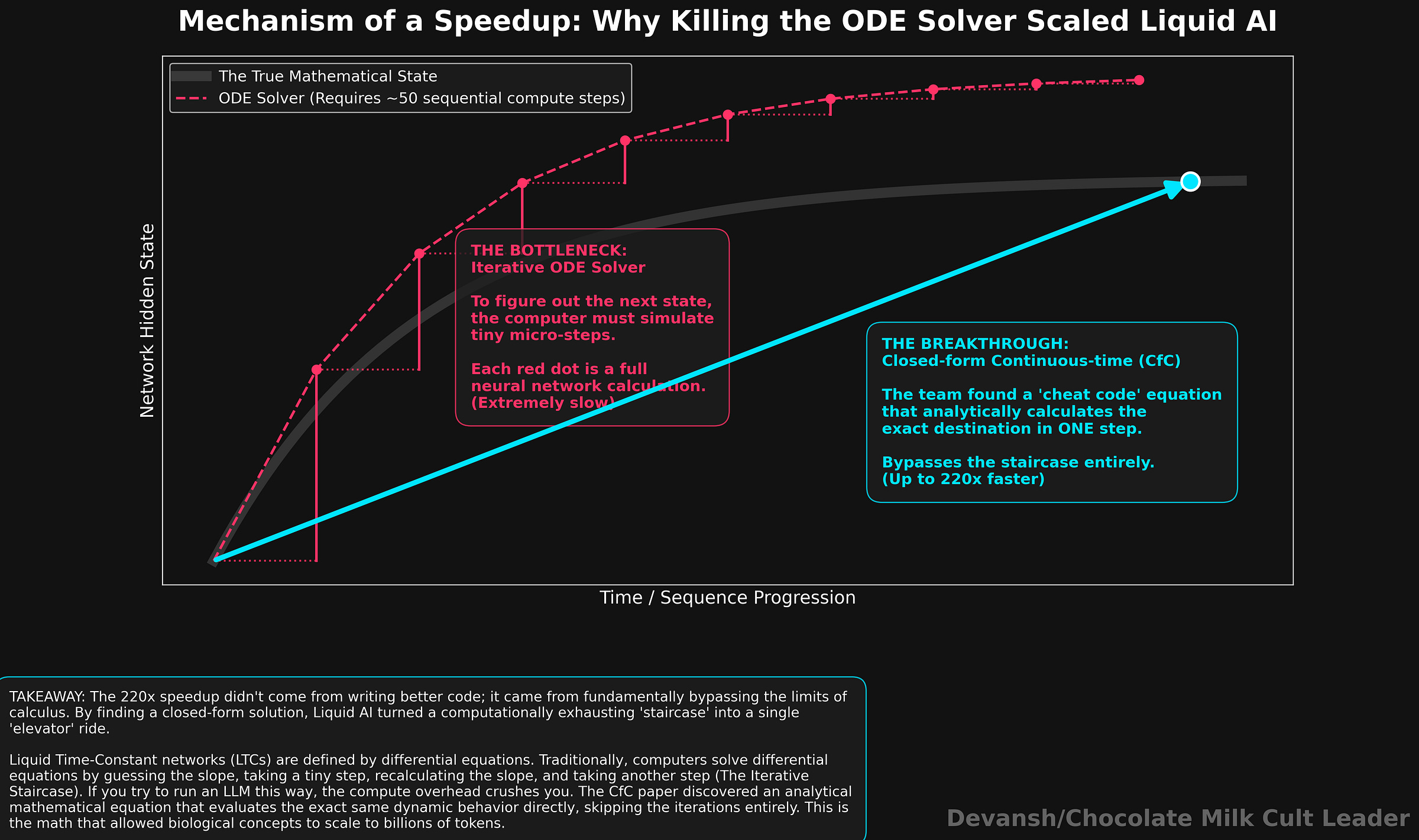
If this architecture was ever going to process billions of tokens instead of just steering a car, they had to kill the ODE solver.
In 2022, they found the cheat code: the Closed-form Continuous-time (CfC) network. They found an analytical approximation that computed the entire dynamic behavior of the system in a single step, bypassing the iterative solver entirely. It preserved the input-dependent adaptability of the worm’s brain, but ran up to 220 times faster.
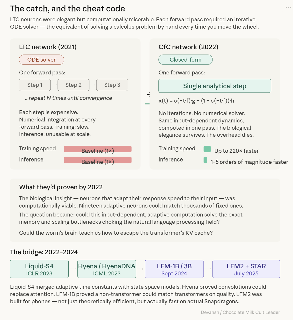
They had successfully separated the biological elegance from the computational overhead. This allowed us to kick things up a notch.
Bridging to the Foundation Model Era
Between 2022 and 2024, the team realized that this adaptive, input-dependent computation could solve the exact memory and scaling bottlenecks choking the natural language processing field.
This led to Liquid-S4, a merge of their dynamic time constants with the State Space Models we discussed in Section 3. They explored Hyena, proving that long convolutions could replace attention for certain sequence tasks.
By September 2024, they released the first generation of Liquid Foundation Models (LFM-1B and LFM-3B). These models proved the foundational thesis: a non-transformer architecture could match the benchmark quality of models like Microsoft’s Phi-3.5, while remaining significantly smaller.
But matching a transformer in a benchmark is not the same thing as surviving in a phone.
The real question was not, “Can we build a non-transformer that is smart?” The real question was, “If we have all these non-transformer operators — SSMs, convolutions, adaptive gates — which exact combination of them actually runs fastest on the hostile silicon of a Snapdragon processor, without blowing up the memory budget?”
To answer that, Liquid AI built a machine to evolve the answer for them. But before we look at the machine, we need to understand the deep design intuition it discovered: Architecture is just budget allocation.
5) The Hybrid Insight: Architecture as Budget Allocation
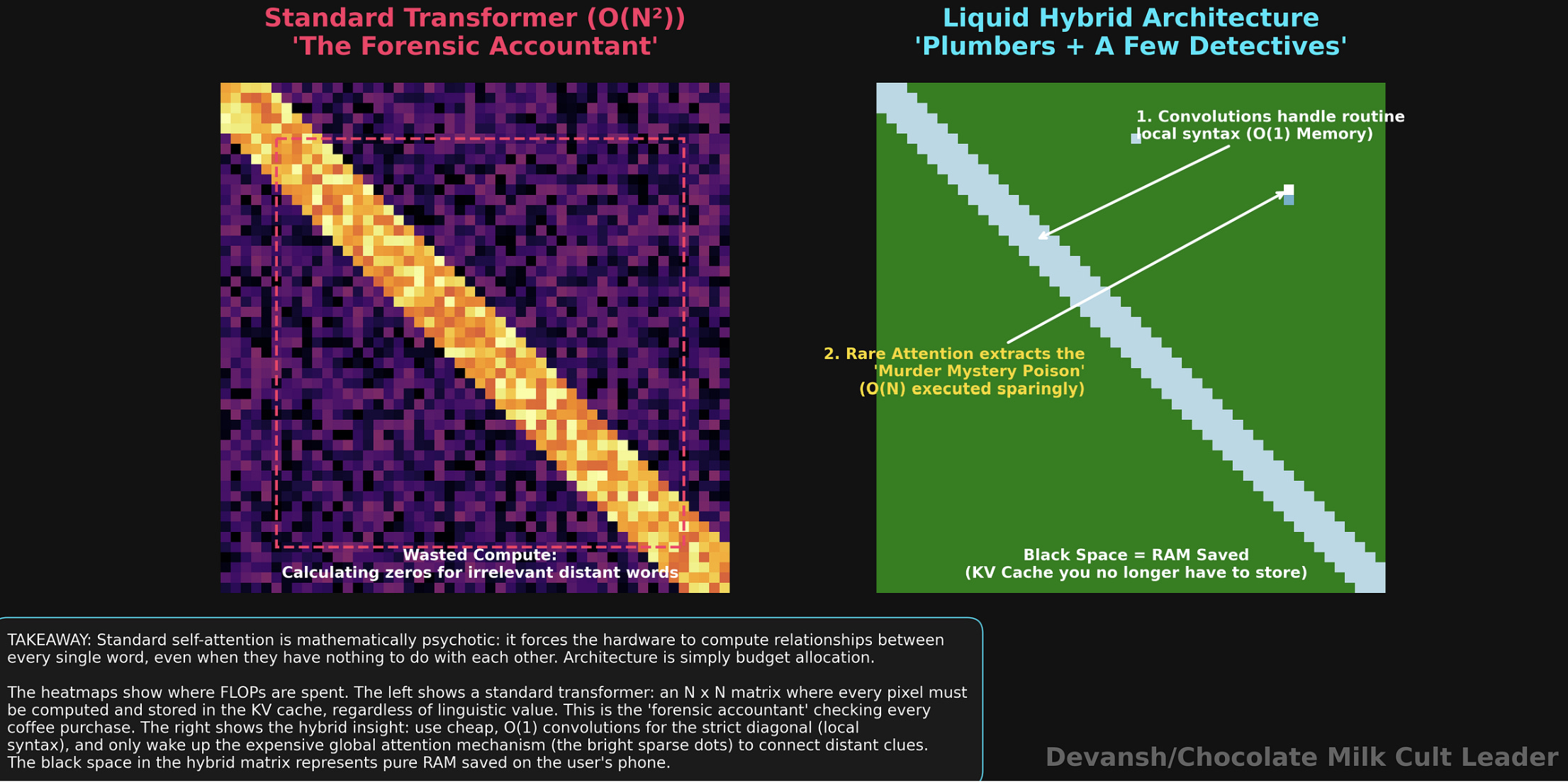
If you step back from all the math and just look at how language actually works, the transformer’s obsession with global attention starts to look a little… obsessive.
Language is overwhelmingly local. If you see the word “The,” you are almost certainly looking for a noun right after it. Most of what a language model does is routine linguistic plumbing — figuring out subject-verb agreement or that “he” refers to “John” in the previous sentence.
Yes, long-range dependencies exist. If page 1 of a murder mystery mentions a specific poison, and page 300 reveals the killer, the model needs precise, global retrieval to connect those two concepts.
But standard self-attention treats every single word like it might be the key to the murder mystery. It pays the maximum possible computational price — the quadratic n squared math and the full KV cache — to compare the word “The” to 32,000 other words, just in case one of them is relevant. It is like hiring a team of forensic accountants to audit your daily coffee purchase.
The Portfolio Allocation
If you accept that most of language is local, the architectural answer becomes incredibly obvious: You take cheap, fast, myopic operators — like convolutions — and use them for the vast majority of the model’s layers. Let them handle the routine syntax. They don’t need a KV cache, and they run blazingly fast on a phone CPU.
Then, you take the expensive, memory-hogging exact retrieval mechanism — attention — and use it sparingly. You only wake it up when you actually need to find the poison on page 1. The ratio between the cheap layers and the expensive layers becomes the master control knob for your entire inference cost.
The Survival Channel
But if 80% of your layers are functionally blind convolutions that only look at the 3 words next to them, doesn’t the model just forget everything else?
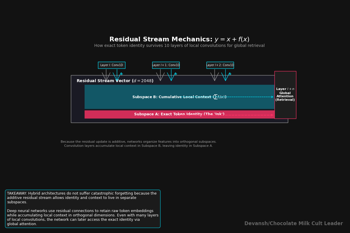
It survives because of the residual stream.
When a token enters the model, its original mathematical meaning is posted to the chat. When a cheap convolution layer processes that token, it doesn’t delete the original meaning. It just figures out some local context and adds that annotation to the chat.
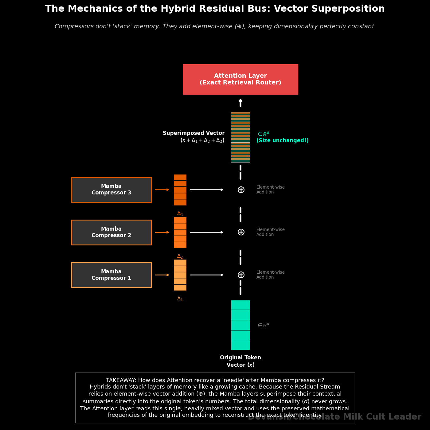
By the time the signal reaches the rare, expensive attention layer, that attention layer can read both the original token identity AND all the local context the convolutions gathered along the way. The convolutions didn’t destroy the signal; they just annotated it.
This is the exact hybrid insight Liquid AI used to build LFM2. How they found their ratios, and the rest of their technical details are all a work of art, which is exactly what we will be looking at next.
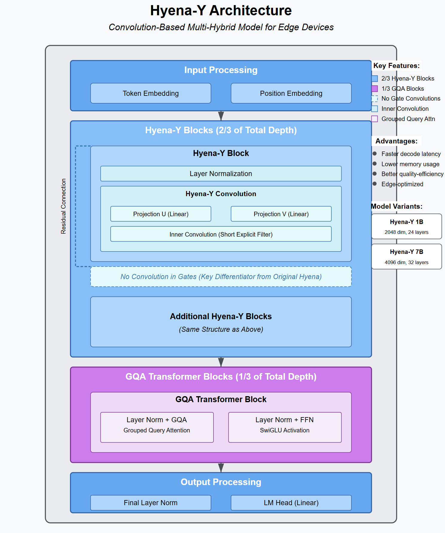
6) What is the Architecture of LFM 2, the best Edge AI Model
Their 10-to-6 split is predicated on the observation that exact global retrieval through self — attention is being dramatically overspent in standard architectures. Most layers in a language model do not need to look at every previous token. They just need to process local patterns cheaply and move on. The expensive global operation should be deployed sparingly, like a specialist you call in for the cases that actually require it, not a default you run in every single layer.
Let’s break this down further. When you think about it, every block in a language model pays for two jobs.
The first is token mixing: letting words talk to each other to absorb context. This is where the transformer’s budget either bleeds out or holds, because standard token mixing is self-attention (the expensive, KV-cache growing tax).
The second job is channel mixing: processing the individual word after it has absorbed context. In LFM2, channel mixing is handled by a SwiGLU feed-forward network, which is a fixed cost and maintains no cache.
So, the entire question of whether an architecture can survive on a phone reduces to one decision: what do you use for token mixing? If you use attention everywhere, you pay the cache tax everywhere. LFM2 found a cheaper token mixer to handle the routine work.
The Gated Short Convolution Block: Adaptivity Without the KV Cache
Remember our observation that most text probably cares about a few local dependencies? This is where is becomes useful.
Most people think that if you want a model that adapts its behavior based on what it is reading, you need attention. Without it, you are stuck with dumb, fixed operations.
People are wrong (shocker).
LFM2 adapts its behavior based on every token it processes without a single byte of KV cache or persistent memory.
Here is how:
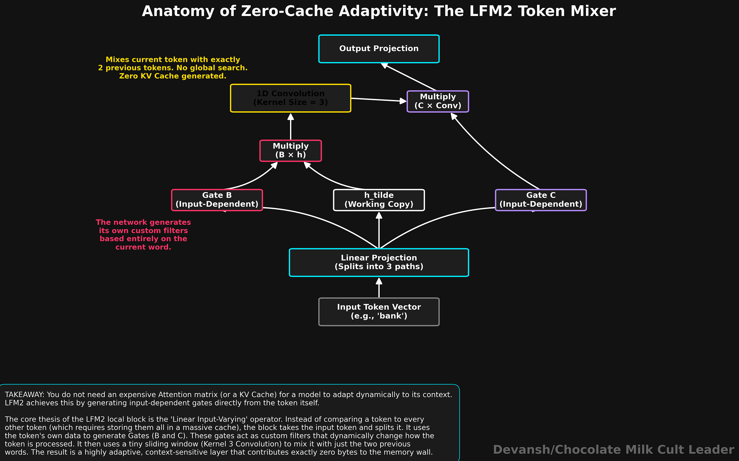
Step 1: Split the input. The incoming token vector is multiplied by a learned weight matrix (a linear projection) to produce three separate vectors: B, C, and h_tilde . h_tilde is the working copy of the token’s information. B and C are gates — vectors of numbers that control signal flow. Critically, B and C are generated directly from the current token’s representation, meaning the model produces different gates for different inputs. The adaptivity is built in at step 1 before any mixing occurs.
Step 2: Apply the first gate. Gate B is multiplied element by element against h_tilde to produce a new vector y. This first gate modulates the signal entering the convolution. Rather than reading “ambiguity,” the network dynamically adjusts its mathematical sensitivity based on the input vector, utilizing Linear Input-Varying (LIV) operators. Adaptive dynamics without the differential equations.
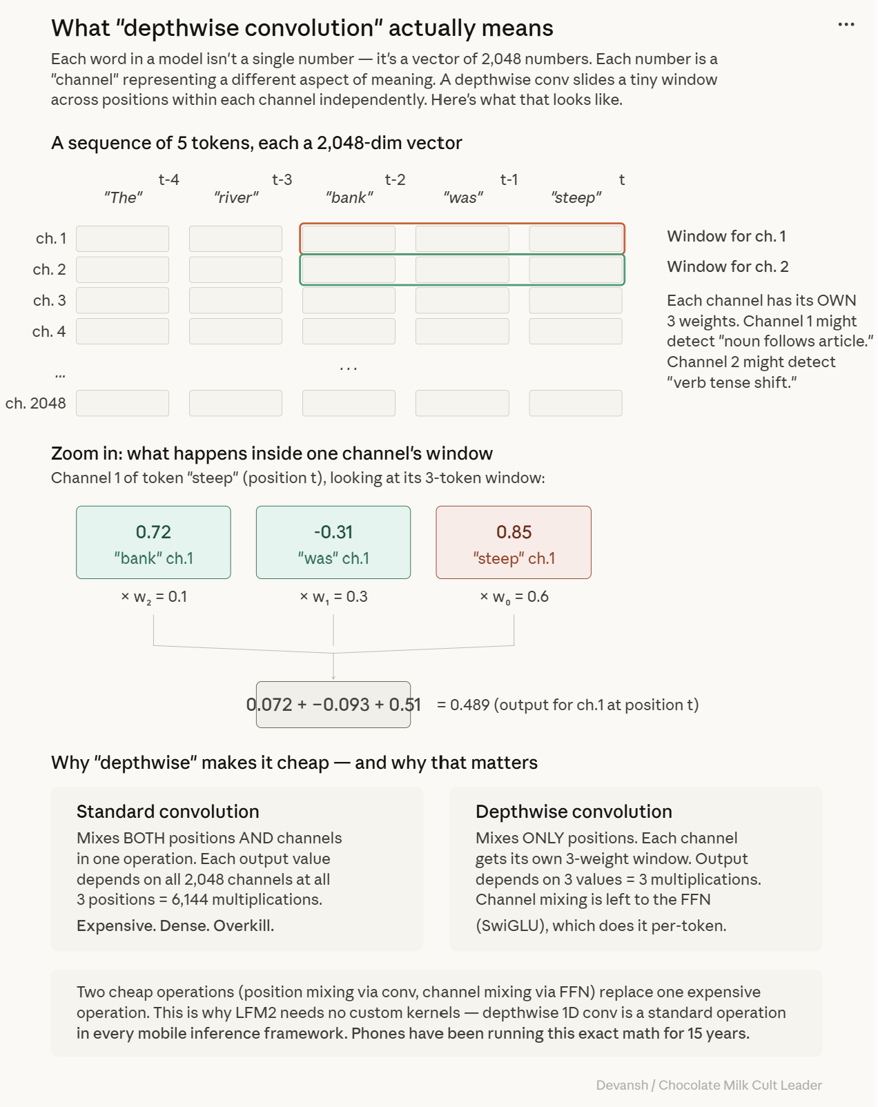
Step 3: The convolution. The gated signal y passes through a depthwise 1D convolution with a kernel size of 3. A 1D convolution acts as a causal sliding window, combining the current token with the two immediately preceding it. “Depthwise” means it mixes positions within each channel independently, but does not mix between channels, deliberately keeping the operation cheap. The math is: z at position t, channel c = (w0 * y at position t, channel c) + (w1 * y at position t-1, channel c) + (w2 * y at position t-2, channel c). This requires three shared weights per channel and maintains a tiny rolling buffer that never grows, ensuring a constant cost per token.
Step 4: The second gate and exit. Gate C is multiplied element by element against the convolution output z. This modulates the exiting signal before it is multiplied by a final weight matrix to map back to the model dimension.
Ten layers of this block provide fully adaptive token mixing with zero persistent memory.
But a kernel size of 3 means the layer is blind to anything four words away. How much of a problem is that really?
Why a Tiny Kernel Size of 3 Actually Works for Language
Liquid AI’s architecture search system (STAR) evaluated multiple kernel sizes. The search consistently rejected broader windows. While a size-64 kernel offered small quality gains, it incurred massive hardware penalties via more multiplications and worse CPU cache efficiency.
This is an empirical finding about language modeling: the mechanical work of processing language — subject-verb agreement, bigram statistics — is overwhelmingly local. Stacking small kernels also naturally grows the effective reach; two size-3 layers in a row allow information to diffuse across five tokens.
More importantly for builders, depthwise 1D convolutions are standard operations across inference frameworks like llama.cpp, ExecuTorch, MLX, and ONNX Runtime. Unlike Mamba, which requires custom associative scan kernels that many mobile stacks lack, LFM2’s local blocks are shippable today.
If ten layers handle the cheap work, the remaining six must justify their memory bill.
The 6 Attention Layers: Paying for the Premium Global Retrieval Service
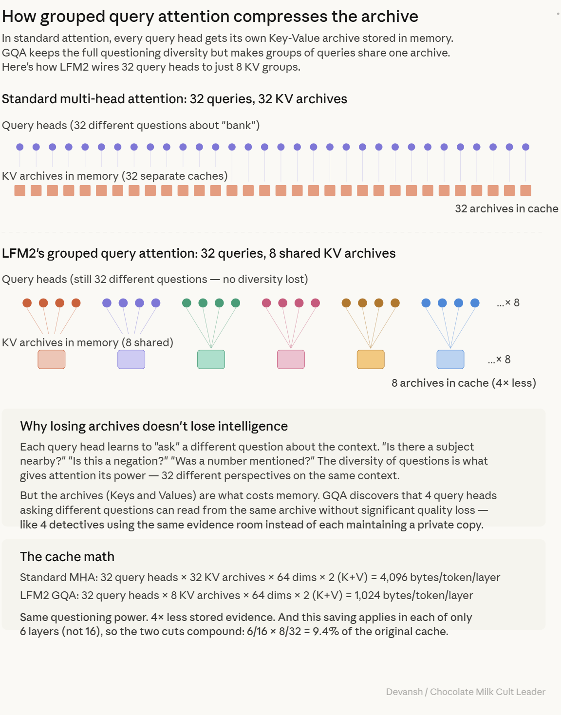
LFM2 retains six grouped-query attention (GQA) blocks where the token can look at every previous token and maintain a KV cache. Standard multi-head attention gives every query head its own private Key-Value archive. LFM2 uses 32 query heads but restricts them to 8 KV groups, meaning every 4 query heads share the same Key-Value archive. This preserves 32 distinct attention patterns while dropping the storage cost by 4x.
Distance is handled by Rotary Position Embedding (RoPE), which rotates query and key vectors so the dot product measures relative distance. The convolution layers require no positional encoding at all, because their three weights are permanently assigned to specific positional offsets. Every component is optimized to lower the final cache math.
To maintain stability downstream of ten convolution blocks, LFM2 applies QK-Norm. Attention scores can grow without bound as training progresses — the model makes queries and keys “louder” over time, and the dot product spikes. The softmax then collapses into a hard winner-take-all that ignores everything except one token. The attention pattern stops being useful.
LFM2 normalizes query and key vectors before the dot product. After normalization, the maximum possible attention score is bounded by the square root of the head dimension — for 64-dimensional heads, that ceiling is 8. This matters specifically because these rescue layers sit downstream of ten convolution blocks accumulating local context. If the attention scores are unstable, the premium service that justifies the entire architecture’s design breaks down exactly when you need it most.
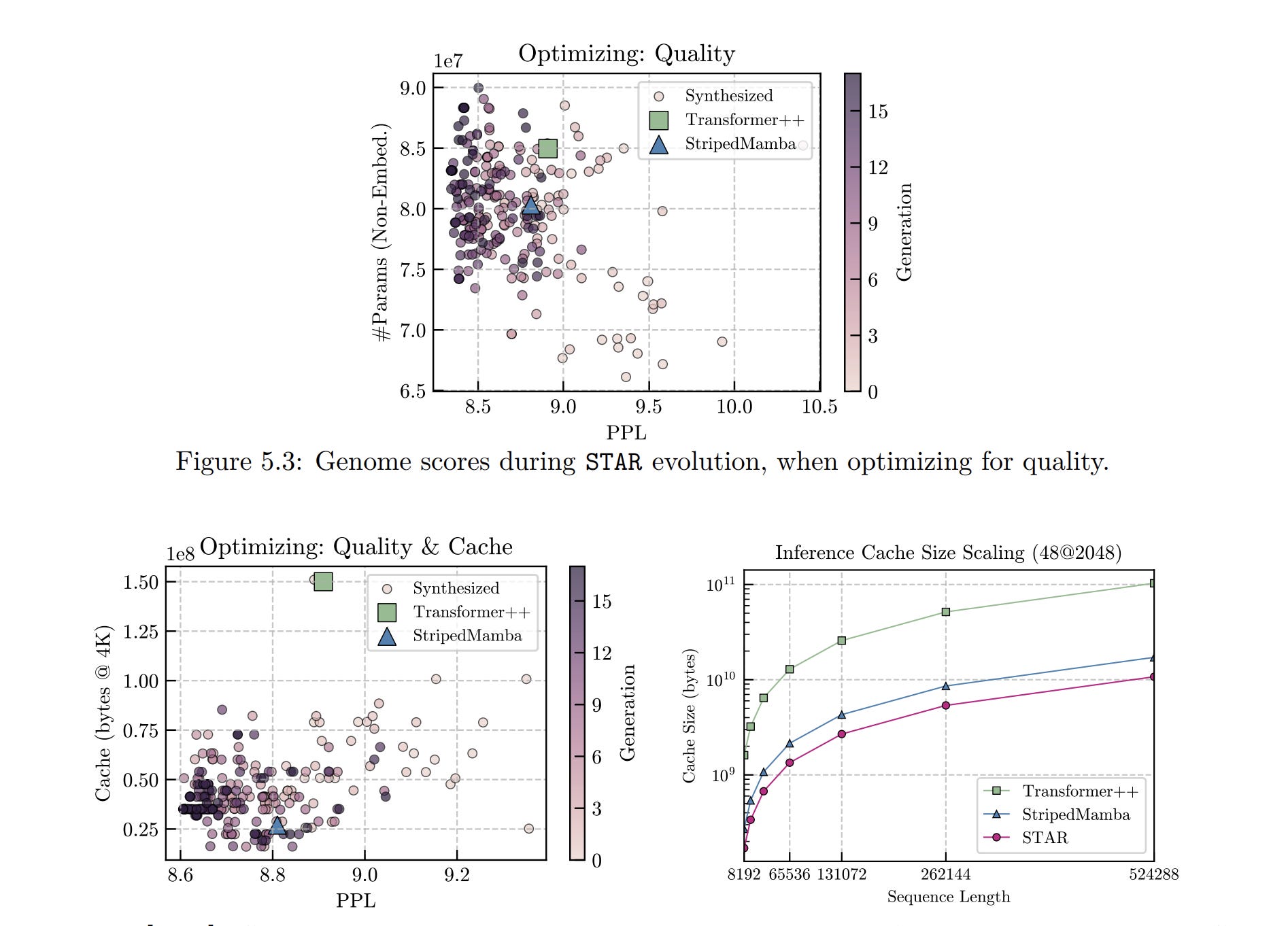
The Actual KV Cache Math: 192 MB vs 524 MB
Here is the formula I’m sure you have imprinted into your psyche by now:Cache per token = 2 * attention layers * KV groups * dimension per head * bytes per element
For LFM2: 2 * 6 layers * 8 groups * 64 dimensions * 1 byte = 6,144 bytes per token. At 32,000 tokens, that is roughly 192 megabytes.
Compare that to Llama 3.2 1B (same groups, dimensions, and precision, but 16 attention layers). That is 16,384 bytes per token, or 524 megabytes at a 32,000 token context.
Running 6 attention layers instead of 16 cuts the cache by 63%. Compare it to a full 16-layer standard multi-head attention stack, and LFM2 stores about 9.4% as much KV memory — a 90% reduction. The memory win compounds sparser attention with cheaper attention.
Turns out, we didn’t need to pay the complete cost of exact retrieval every layer.
But this chindi behavior creates a terrifying mechanistic problem.
How Information Survives the Blind Layers: Residual Connections
If ten layers can only see three tokens, how does a fact from 100 tokens ago survive long enough for an attention layer to retrieve it? Why doesn’t the representation turn into local soup before a rescue layer arrives?
The answer is residual connections.
If a layer simply completely transformed its input, early information would be destroyed immediately. Residual connections prevent this with an additive rule: output = input + Layer(input). The layer computes something and adds it on top of what came before. The raw token identity is always mathematically present in the stream because it was never subtracted out. Dimensional separation in the 2048-dimension vector allows the token identity and the local context annotations to broadcast on different frequencies without destroying each other.
Evidence suggests that after 4 to 8 consecutive blind layers, verbatim needle-in-a-haystack recall dies. Local annotations eventually contextualize the representation so heavily that exact identity becomes hard to recover. LFM2 spaces its 6 attention layers out to roughly one every 2.7 blocks, keeping it in the safe zone.
This is the explicit tradeoff. For forensic citation of 100,000-token documents, this architecture will underperform a pure transformer. But for on-device conversations, working ambiently (which means a lot of irrelevant tokens coming in), summarization, and agentic tool use, it dominates.
As alluded to earlier, Liquid AI didn’t just guess this exact 10/6 configuration. They built a machine to mathematically evolve the answer on actual phones under real constraints. That machine is called STAR, and its long-term value is stronger than any single model it produces. Instead of getting super into the nitty gritties, we will transition to exploring that now.
7) How STAR Works: The Architecture Search Machine
The 10 convolution layers. The 6 attention layers. Kernel size 3. Eight KV groups. The exact spacing of the rescue layers. None of that was guessed. Nobody sat in a room and had an inspired glasses being pushed up epiphany where the optimal edge architecture descended from heaven.
Hand-designing an AI architecture is, at best, an educated guess constrained by human intuition. When AI21 designed Jamba, they ran ablations comparing a 1:7 attention-to-Mamba ratio against a 1:3 ratio, found little quality difference, and picked 1:7 because it was more compute-efficient. That is better than guessing blind, but it is still a manual search through a tiny slice of the design space, limited to the clean ratios a human thought to test. However, the right architecture for a Samsung phone might be completely different from the right architecture for an AMD laptop, and neither is likely to be a clean ratio that looks good on a whiteboard.
Liquid AI built a search machine to do the embarrassing part: brutally test architectural ideas on real hardware until most of them die.
That machine is STAR (Synthesis of Tailored Architectures). If you are trying to understand what is actually durable about Liquid AI, STAR matters more than any individual 1.2B model ever will. Models age fast. Benchmarks move. But a system that takes a hardware target, a latency budget, a memory ceiling, and a quality suite, then mathematically evolves the architecture that best fits that exact regime? That is not one good model. That is a factory for good models.
Why Hand-Designing Architectures is a Deployment Hazard
Even for a 16-layer model, the possible configurations of operators, sharing patterns, expansion factors, and featurizers are endless. A researcher can explore maybe a dozen configurations in a focused effort. STAR evaluates entire populations across generations.
When the hardware target changes — say, from a Snapdragon 8 Gen 3 to a Gen 5 — the optimal architecture may shift in ways no human would predict because the cache hierarchy changed or the compiler handles operations differently. A researcher has to start over with new intuitions. STAR simply reruns the search.
There is also the bias problem. Researchers optimize for elegance. They gravitate toward architectures that have nice theoretical properties, look clean in a diagram, and make for a good NeurIPS oral presentation. Hardware does not care about elegance. Hardware only cares whether the operations map efficiently to its execution units. STAR has no aesthetic preferences; it only knows what is fast, what is small, and what scores well.
But to search this vast space effectively, you need a common mathematical language that can express all major sequence operators inside the same geometry. This is harder than you’d think, and why we need to really abstract things well (which makes me think that studying category theory might lead to some interesting breakthroughs for AI, especially for more meta-level work).
The LIV Abstraction: One Algebra for Every Architecture
STAR’s search space is built on a theoretical foundation called the Linear Input-Varying (LIV) operator.
In plain terms, an LIV operator produces its output by multiplying the input sequence by a linear transformation, but that transformation is itself generated from the input: Output = T(x) * x, where T is a matrix that depends on the input x.
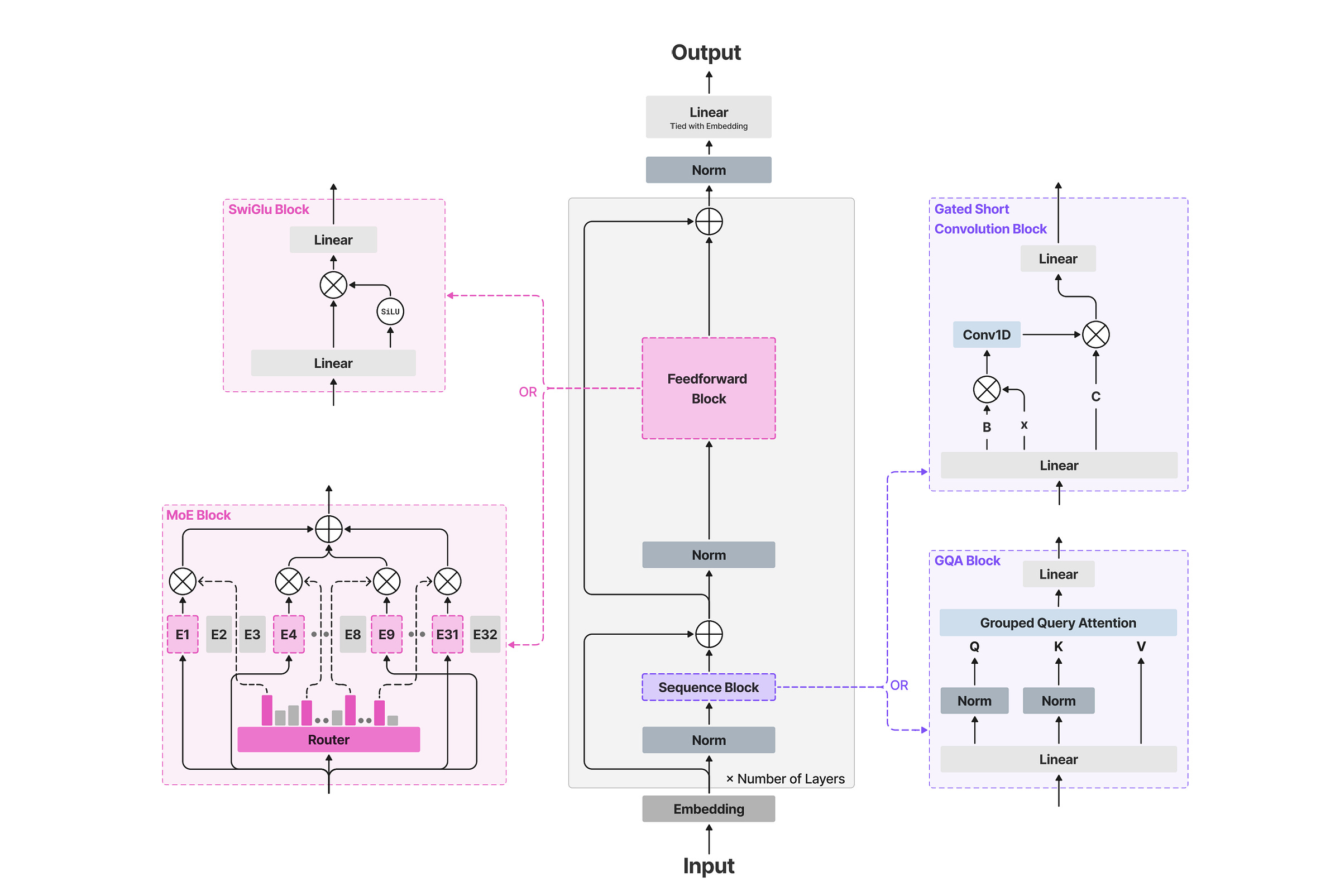
What this buys the search system is total algebraic unification. It expresses attention, linear attention, state space models, convolutions, and gating operators as special cases of the exact same family:
If
T(x)is the softmax attention matrix built from query-key dot products, you get standard self-attention.If
T(x)has the structured form of a state-transition operator, you land in Mamba territory.If
T(x)is Toeplitz-structured with learned, input-dependent gating, you get LFM2’s gated convolution.
These terms might be a bit intimidating to you, so here is a visual that walks you through the same. It’ll make understanding this stuff a lot easier.
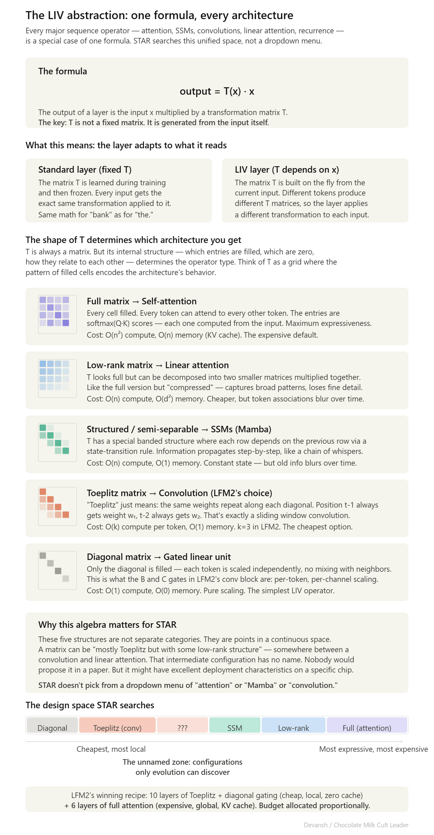
Because STAR moves through a continuous mathematical geometry rather than picking between discrete labels, it can discover intermediate or mixed structures that no human would have proposed. This turns the space between “convolution” and “SSM” from a vacuum to a rich set of unnamed configurations with (potentially) excellent hardware behavior.
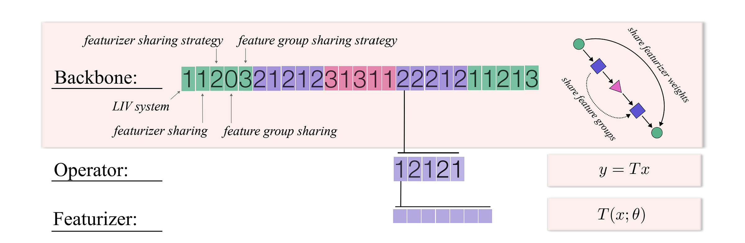
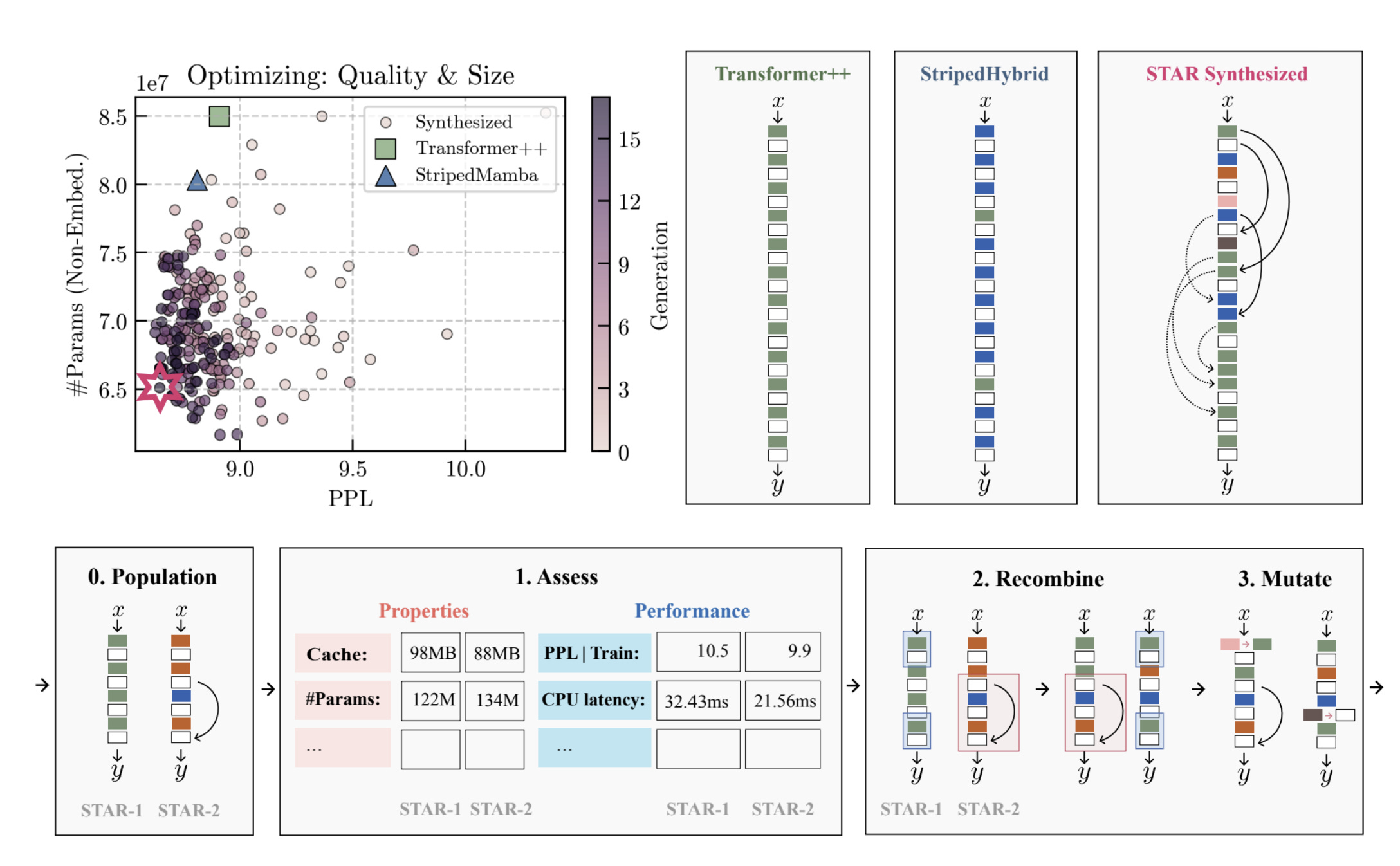
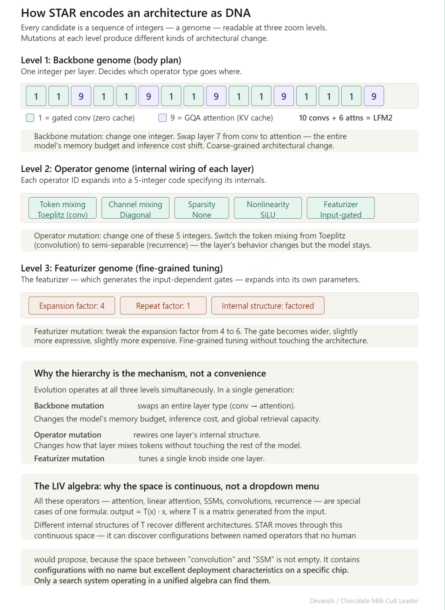
The Architectural Genome: Evolving at Three Resolutions
To work effectively, STAR encodes every candidate architecture as a hierarchical genome — a sequence of integers describing the architecture at multiple scales simultaneously:
Backbone Genome (Macro): One operator ID per layer. This decides the body plan — what kinds of blocks appear and where.
Operator Genome (Wiring): Expands the operator ID into a short code specifying the token mixer, channel mixing pattern, and nonlinearity.
Featurizer Genome (Micro): Defines expansion factors, repeat counts, and internal sharing patterns. These are the tiny choices that quietly determine whether a model ships or crashes.
This hierarchy allows evolutionary search to work at multiple resolutions. A mutation can swap whole operator types across layers, rewire one specific layer, or tune fine-grained details without disturbing the broader architecture.
Multi-Objective Evolution on the Pareto Frontier
STAR uses gradient-free evolutionary algorithms to optimize across multiple objectives simultaneously. It maintains a population of candidates, evaluates them, keeps the ones that are not dominated by any other candidate, and breeds them for the next generation.
This setup helps a lot when it comes to balancing multiple factors. When it comes to edge deployments, quality, latency, and memory must be threaded together. A model that wins on perplexity but blows the memory budget is useless. STAR navigates the synthesis by tracking the Pareto frontier — the exact set of architectures where you cannot improve one objective without degrading another.
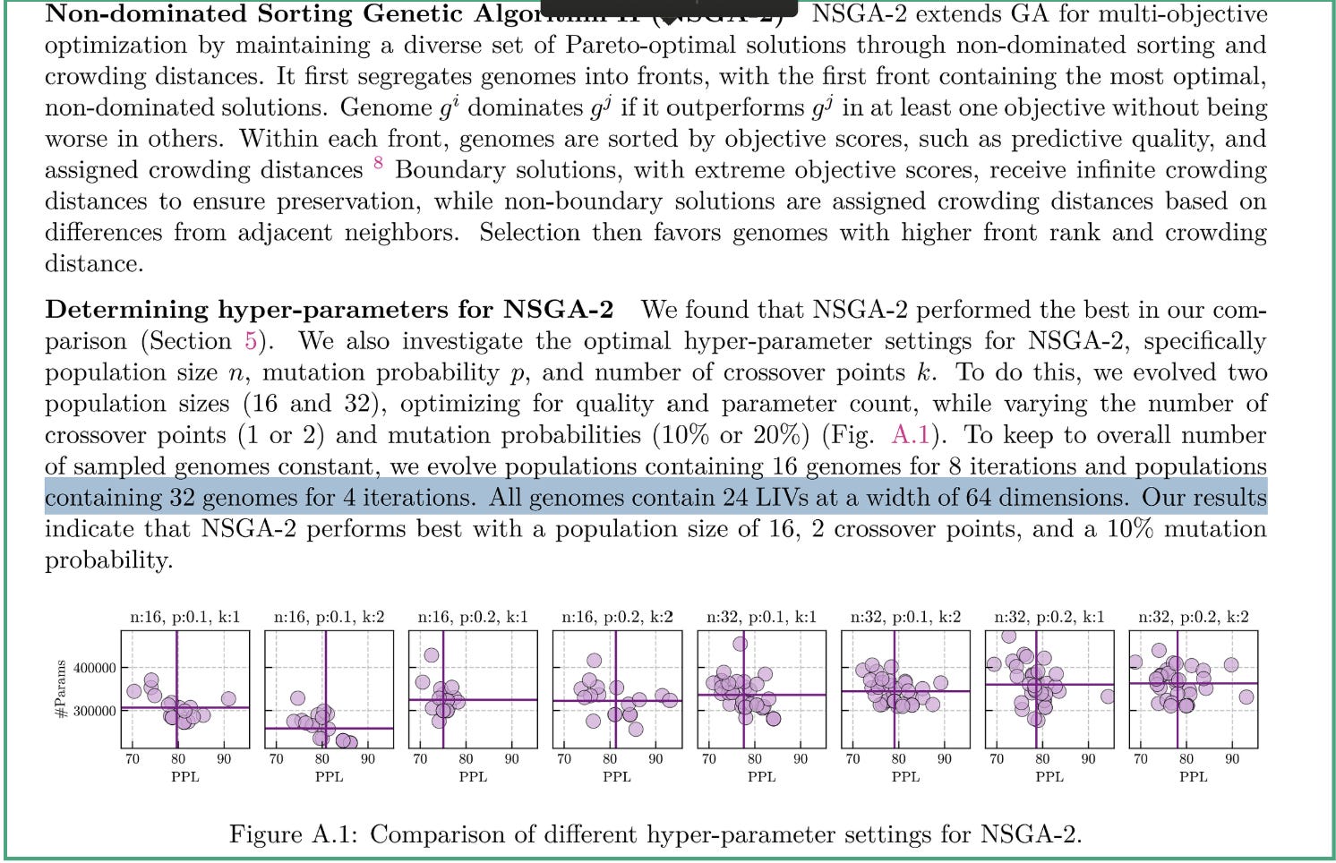
“Given the wide range of possible applications of current AI systems, enabling systematic and automatic optimization of model architectures from the multitude of existing computational units is key to meeting the various demands these applications pose, in terms of efficiency (e.g., model size, inference cache size, memory footprint) and quality (e.g., perplexity, downstream benchmarks), and a prerequisite on the path to further, consistent improvements on the quality-efficiency Pareto frontier.”
Most evolved architectures outperformed hand-designed hybrids within just a few rounds of evolution. But despite these amazing results, this OG wasn’t good enough. Getting to LMF2 required an upgrade.
“Our earlier academic prototype (STAR) (Thomas et al., 2024) explored a specific design space of operator/layout choices with an evolutionary search heuristic optimized on proxy signals (i.e., perplexity for quality, cache size for efficiency). In practice, these proxies do not transfer reliably to downstream task scores or device-level latency and memory, limiting their utility as optimization objectives. By contrast, the LFM2 pipeline centers the objective: downstream task scores and hardware-in-the-loop TTFT/latency/memory on release runtimes. In practice, we found this has a much larger impact than the particulars of the search space or choice of search heuristic.”
The LFM2 Pivot: Why Liquid AI Replaced Proxies with Hardware-in-the-Loop
The original STAR paper optimized against proxy signals: perplexity for quality, and estimated cache size for efficiency. The LFM2 technical report is blunt about why they abandoned this: proxy metrics lie.
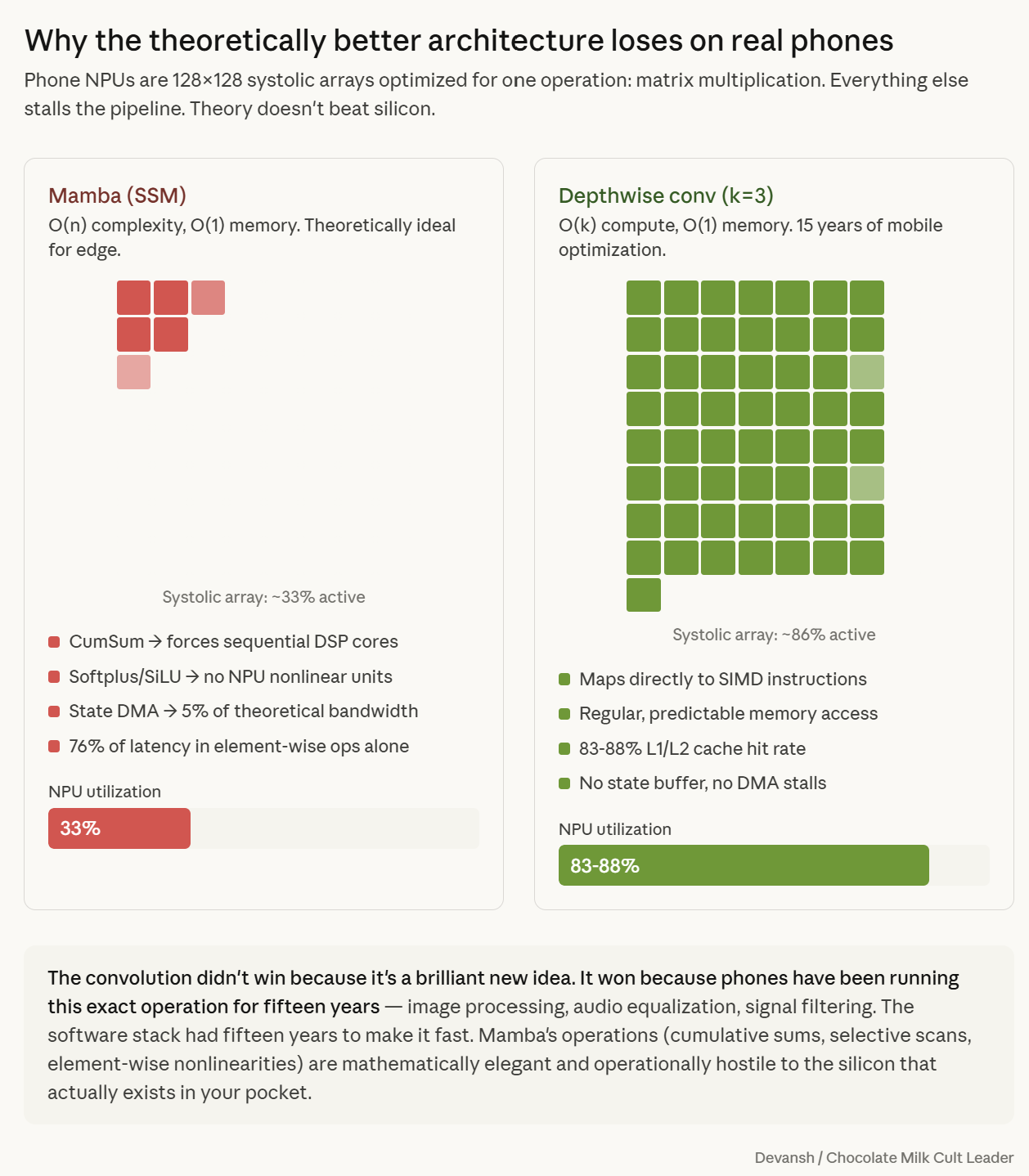
A Mamba layer and a convolution layer might have similar theoretical FLOPs, but Mamba requires sequential scan operations that stall the CPU pipeline, while convolutions map to highly optimized SIMD instructions. Theoretically, better performance will lead to worse outputs IRL.
Likewise, estimated cache size ignores activation buffers, framework overhead, and allocator behavior. The only metric that tells you if a model will crash a device is peak RSS — the actual physical memory the process consumes at its worst moment. This is something you have to get your hands dirty to measure.

The LFM2 pipeline fixed this by dragging the search onto real devices. Every candidate architecture is compiled into deployment format (llama.cpp or ExecuTorch) and loaded onto actual hardware: either a Samsung Galaxy S24 Ultra and an AMD Ryzen laptop to get both ends. They are profiled at batch size 1 across both 4,000 and 32,000 token contexts. Candidates that violate device-side budgets for time-to-first-token, decode latency, or peak RSS are instantly discarded.
This kind of search is extremely powerful, but it comes with a massive downside — it’s very very expensive. t requires thousands of GPU-hours for proxy training and a dedicated physical device lab for continuous profiling.
Google DeepMind, OpenAI, Anthropic, Chinese labs, Apple, and Meta all possess the capital and internal frameworks to replicate hardware-in-the-loop search. Liquid AI’s success depends on converting that lead into ecosystem lock-in through runtimes, developer tooling, and accumulated profiling data — before a hyperscaler decides to look into doing this. This means they need to move quickly; anything that can block them has to go.
And understanding this leads to understanding one of their most surprising design outcomes.
Why STAR Completely Rejected SSMs
For all their theoretical elegance, STAR completely rejected State Space Models for Edge Deployments.
Every major SSM variant was available in the search space. The LFM2 report explicitly lists S4, Mamba, Mamba-2, Liquid-S4, and S5 as candidates. STAR simply chose not to include them. The hardware-in-the-loop search repeatedly selected the minimal hybrid of gated short convolutions and grouped-query attention, ruthlessly excluding SSMs from the surviving architectures.
If you’ve read our prior deep dives and followed along with the journey, the reasons might be clear to you. So instead of repeating stuff, here is a little visual that you can save to remember the details on the go —
This lays all the goundwork for us to finally understand Liquid’s newest model.
8) How Does Liquid AI Train Small Models to Compete With Much Larger Ones?
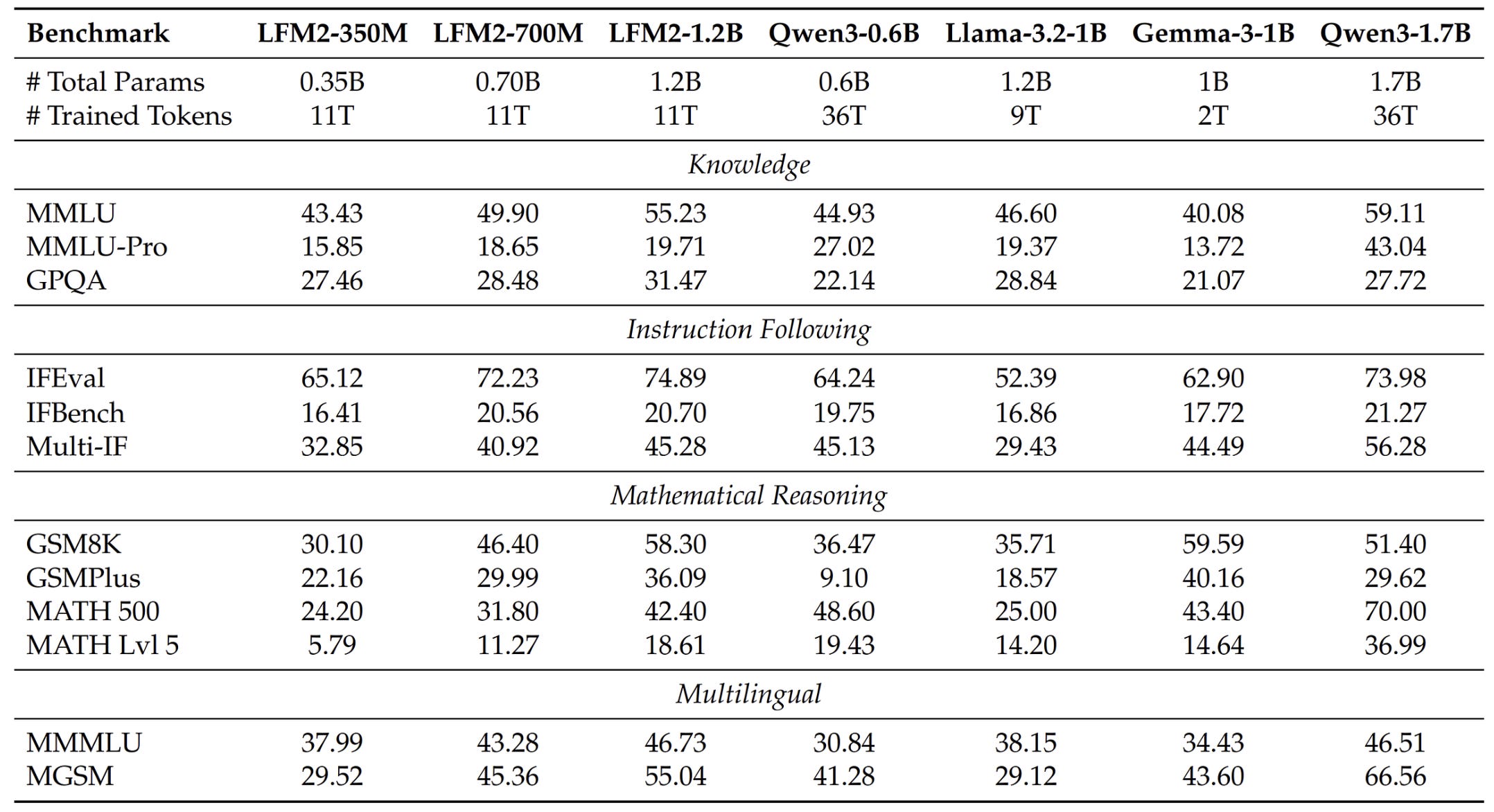
LFM2.5–1.2B matches or beats Qwen3–1.7B — a model with 42% more parameters — on multiple benchmarks. Let’s understand the four specific training innovations that make this happen.
How the Student Model Learns From a Bigger Teacher Without Storing Everything
Knowledge distillation trains a small model (the student) to mimic a large model (the teacher). Instead of just learning to predict the correct next token, the student learns to match the teacher’s full probability distribution — not just “the answer is X” but “X is most likely, Y is a decent second choice, Z is plausible, everything else is garbage.” That ranking information makes the student significantly smarter than learning from raw data alone.
LFM2 models are distilled from LFM1–7B. The problem is storage. The teacher’s full distribution over a 65,536-token vocabulary for every position in a multi-trillion-token corpus would require petabytes. Liquid AI stores only the top 32 logits per token — a 2,000x compression.
But truncation breaks the standard training math. Here’s why.
The standard way to measure how well the student matches the teacher is called KL divergence — it’s essentially a score that says “how different are these two probability distributions?” Lower score means the student is mimicking the teacher well. Higher score means it’s off.
To help the student learn, you typically apply temperature scaling — which smooths out the teacher’s predictions so they’re less extreme. Instead of “token X has 90% probability and everything else is near zero,” temperature scaling softens it to something like “token X has 40%, Y has 25%, Z has 15%…” This makes the ranking information easier for a small model to absorb.
The problem: when you only stored 32 out of 65,536 tokens and then apply temperature scaling, the math tries to spread probability to all 65,536 tokens — including the 65,504 you have no teacher data for. The loss function is trying to match a distribution that doesn’t exist. Training becomes unstable. The model oscillates instead of learning.
Liquid AI’s fix splits the matching problem into two separate parts:
Term 1: Membership loss. How much total probability mass should the student assign to the teacher’s top-32 tokens versus everything else? A binary comparison. No temperature scaling — because temperature applied to a truncated distribution would smooth probability toward tokens you have zero information about.
Term 2: Conditional ranking loss. Within those top-32 tokens, how well does the student match the teacher’s relative ordering? This term gets temperature scaling, because both distributions are defined over the same 32 tokens. No mismatch.
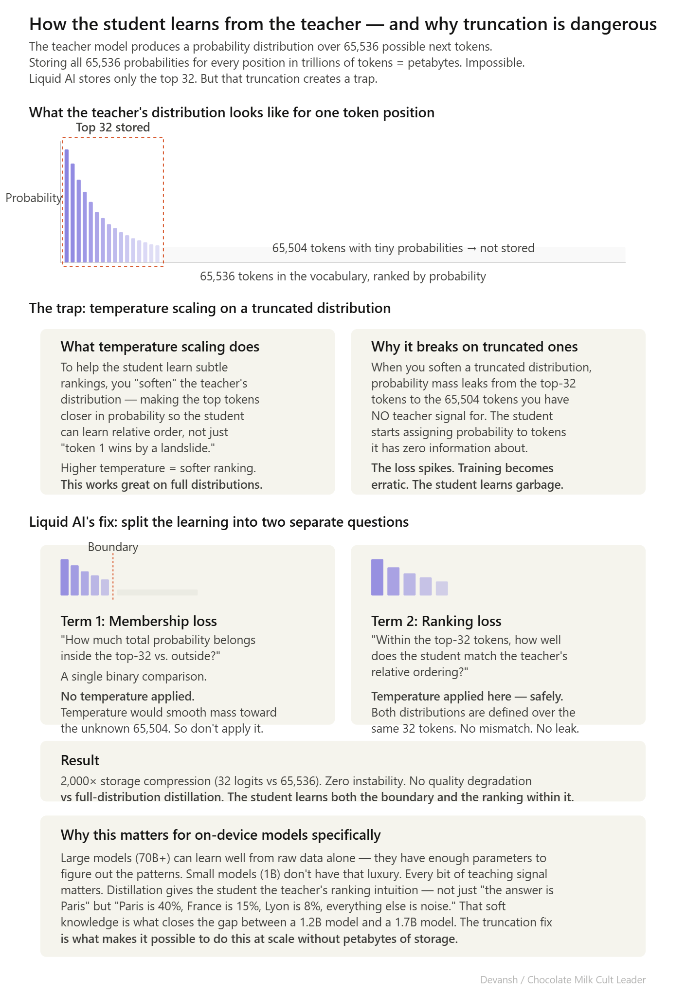
At temperature 1, this decomposition is provably a lower bound on the full KL divergence — the full KL decomposes into three terms (binary, conditional top-K, conditional tail), and dropping the non-negative tail term can only decrease the total. At higher temperatures, the loss becomes a tempered surrogate with a smoother optimization landscape.
This leads us to the next phase of training.
Why Training Examples Are Ordered From Easy to Hard
A 1.2B model has limited capacity. Hitting it with the hardest training examples before it has learned basic patterns produces noisy gradients and wasted compute. LFM2’s supervised fine-tuning stage orders examples from easy to hard.
Difficulty is scored by an ensemble of 12 models ranging from 350M to 235B parameters. For each question, the ensemble computes the fraction that answered correctly. High fraction = easy. Low fraction = hard. Training proceeds from easy to hard using a predictive model to rank questions by estimated difficulty.
Difficulty is measured externally by the ensemble, not by the student’s own performance. This avoids the circularity that kills self-paced learning: a poorly trained student misjudges what’s hard, avoids exactly the examples it needs, and stays poorly trained.
Three Stages of Post-Training: Fine-Tuning, Preference Alignment, and Model Merging
After pretraining on 10 to 12 trillion tokens, the model goes through three post-training stages (in case you’re wondering, this is a massive pretraining budget; and is likely why the model has really good knowledge and capabilities; 2.5 pushed this to 28 Trillion, which validates this assumption).
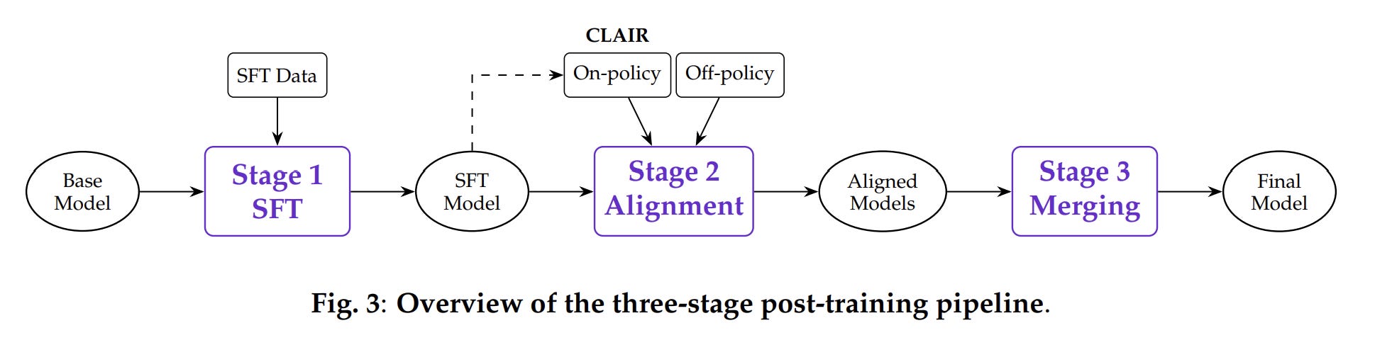
Stage 1: Supervised Fine-Tuning (SFT). 5 to 9 million training examples across 67 to 79 data sources. Roughly 27% general-purpose, 17% instruction following, 13% retrieval-augmented generation, 10% tool use, remainder split across code, math, multilingual, and domain-specific tasks. 80% English, 20% multilingual.
Stage 2: Preference Alignment via DPO. The model generates 5 candidate responses per prompt. An LLM judge scores them. The best and worst form preference pairs. Direct Preference Optimization trains the model to increase the probability of preferred responses and decrease dispreferred ones.
Two details matter for small models.
The KL regularization coefficient (beta) is 5.0 — roughly 10x higher than typical DPO (0.1 to 0.5). A 1.2B model can’t afford to deviate far from its SFT-trained behavior without catastrophically degrading general capabilities. The high beta constrains the optimization to targeted improvements.
Length normalization is equally important — without it, DPO biases toward shorter responses because longer completions accumulate more log-probability, making them look worse regardless of actual quality.
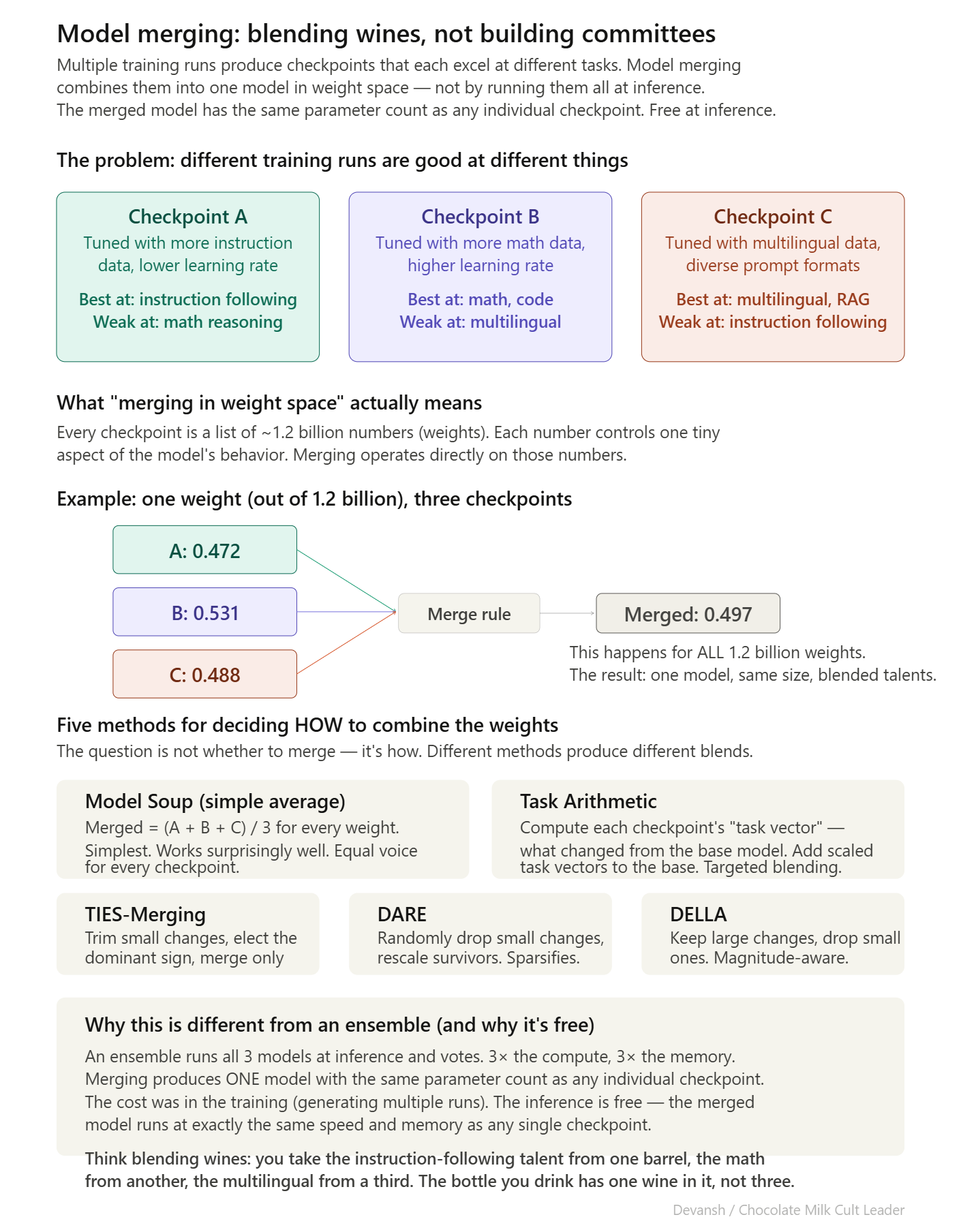
Stage 3: Model Merging. Multiple candidate checkpoints are generated by varying hyperparameters and data mixtures. Each excels in different areas. The best checkpoints are combined into a single model using weight-space averaging.
Five merging methods are tested: linear averaging (Model Soup), Task Arithmetic, TIES-Merging, DARE, and DELLA. Each handles the combination differently — some average all weights, some merge only the weights that changed most, some randomly drop small changes and rescale. The best merged model is selected on a comprehensive benchmark suite. Merging costs nothing at inference — the output is one model with the same parameter count as any individual checkpoint.
Why Liquid AI Quantizes During Training, Not After
All LFM2 and LFM2.5 models are trained with INT4 quantization in the loop from the start. The model learns to produce good outputs despite rounding errors, rather than being trained at full precision and then compressed (post-training quantization). This matters more for small models — a 70B model has enough redundancy that quantization noise barely registers. A 1B model has no slack. Every parameter is working harder, and rounding any of them introduces proportionally more damage.
Conclusion: Where Does Edge AI Go Next
We didn’t spend eight sections tearing apart cache math and evolutionary algorithms just to marvel at a clever 1.2B model. Liquid AI is merely the diagnostic tool. The real story is that the entire trajectory as edge AI and all of it’s implications unfold. However, this is a completely different computing paradigm, with it’s own problems that we musst all be ready to solve.
The Signal-to-Noise Crisis: Learning to Ignore
Right now, if you type a prompt into ChatGPT, 100% of those tokens are intentional. You wrote them. The model assumes every word matters. Even with typos and misspellings, the signal to noise ratio in your input is very high.
Ambient computing is the exact opposite. If an AI is listening to your microphone for 8 hours a day, 99% of what it hears is useless garbage. It hears you typing, a siren outside, small talk about the weather, and someone clearing their throat. Maybe 1% of those tokens are a concrete task or an important decision.
If you feed 8 hours of ambient noise into a standard transformer, it will dutifully calculate exact global attention scores for the siren and the throat-clearing, filling up its KV cache until the phone crashes. Or it will find ways to bill you for the Raja Raja Raja song you played 10x in a row.
All this means the next major architectural leap in edge AI won’t just be about cheaper math. It will be about active ignoring. Just like the human brain filters out the feeling of your shirt against your back so you can focus on reading this sentence, edge models will need adaptive compute mechanisms that instantly classify and discard useless tokens before they ever reach the expensive layers. The architecture will have to shift from “how efficiently can I process this context?” to “how aggressively can I refuse to process this context?”
The Hardware Fragmentation Problem: The Case for Open Standards
The data center is a monoculture. If you write your model in CUDA, it will run beautifully on an NVIDIA GPU, which is what every hyperscaler uses.
The edge is a chaotic wasteland.
There is no “standard” edge hardware. A Snapdragon NPU handles memory differently than an Apple Neural Engine, which handles operations differently than an AMD Ryzen CPU. As Liquid AI’s STAR system proved, the optimal architecture for one phone might run like garbage on a laptop. There are a million different Pareto frontiers.
If you are a startup or a smaller AI team, you cannot afford to build a dedicated hardware-in-the-loop search system to evolve a custom architecture for every single Android device on the market.
This fragmentation forces a strategic fork in the road. Either the massive players (Apple, Google) completely capture the edge because they own the vertical hardware stack and can optimize perfectly for it, OR the open-source community is forced to consolidate around open standards. We will likely see a push for unified inference runtimes and open hardware-profiling datasets. Smaller players will have to pool their testing resources, effectively building a communal “STAR” system, just to survive the hardware chaos.
Unlocking Hostile Markets
Finally, the obsession with edge AI isn’t just about saving battery life on a smartphone. It is about unlocking entirely new markets that are fundamentally hostile to GPUs.
There are massive sectors of the global economy where you cannot just “ping the cloud.” For the last three years, these industries have been locked out of the generative AI boom because the models required server racks they weren’t allowed or able to use.
Architectures like LFM2 change the math. When you can run a highly competent, reasoning-capable model locally in 700 megabytes of RAM, you bypass the cloud entirely. You bring the intelligence to the data, instead of trying to drag the data to the intelligence.
The transformer won the last decade because it was perfectly adapted to the data center — an environment where memory is treated as infinite. The architecture that wins the next decade will be the one that understands memory is a hostage negotiation. And the companies that master that negotiation are about to put AI into everything.
Thank you for being here, and I hope you have a wonderful day,
Dev <3
If you liked this article and wish to share it, please refer to the following guidelines.
That is it for this piece. I appreciate your time. As always, if you’re interested in working with me or checking out my other work, my links will be at the end of this email/post. And if you found value in this write-up, I would appreciate you sharing it with more people. It is word-of-mouth referrals like yours that help me grow. The best way to share testimonials is to share articles and tag me in your post so I can see/share it.
Reach out to me
Use the links below to check out my other content, learn more about tutoring, reach out to me about projects, or just to say hi.
Small Snippets about Tech, AI and Machine Learning over here
AI Newsletter- https://artificialintelligencemadesimple.substack.com/
My grandma’s favorite Tech Newsletter- https://codinginterviewsmadesimple.substack.com/
My (imaginary) sister’s favorite MLOps Podcast-
Check out my other articles on Medium. :
https://machine-learning-made-simple.medium.com/
My YouTube: https://www.youtube.com/@ChocolateMilkCultLeader/
Reach out to me on LinkedIn. Let’s connect: https://www.linkedin.com/in/devansh-devansh-516004168/
My Instagram: https://www.instagram.com/iseethings404/
My Twitter: https://twitter.com/Machine01776819
This is one of the best breakdowns of the on-device memory bottleneck I've read. The KV cache math alone should be required reading for anyone pitching "edge AI" products.
From the IoT side, the signal-to-noise problem you flag at the end is the real unlock. We work with multi-sensor edge gateways that ingest ambient telemetry 24/7 -- temperature, vibration, RF signal quality, device logs. Easily 95% of those tokens are noise. Today we solve it with dumb heuristic filters before anything hits a model, but the idea of architectures that can natively refuse to process irrelevant context is exactly what the next generation of smart edge devices needs.
The hardware fragmentation point also hits hard. We see this constantly across Qualcomm, MediaTek, and even custom RISC-V silicon in industrial IoT. The fact that STAR rejected every SSM variant once real device profiling was in the loop is a massive signal -- theoretical FLOPs mean nothing if the silicon can't execute the operations efficiently.
Curious: do you see the STAR approach eventually becoming an open standard, or does Liquid AI's moat depend on keeping that search infrastructure proprietary?
mind boggling and OHT :)